The 2nd homework assignment has been graded and was returned in
class today. A new
assignment was handed out (there are three problems for
students enrolled in the graduate (589) version of the class ,
only two for the undergraduate (489) students. This new
assignment is nominally due in one week. I would suggest
reviewing the second part of the Feb.
02 notes (E field measurements in clouds) before working on
the 1st problem and the Feb. 06 notes before tackling Questions #2
and #3.
A good portion of the class had a little trouble with parts of
Question #1 so here are a couple of comments.
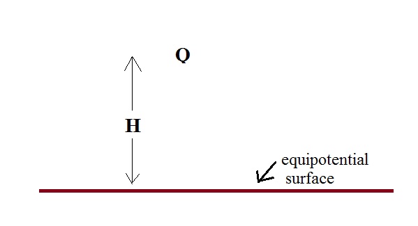
For many it was a question of how to start the problem. We
start with a charge Q positioned a distance H above the surface of
the earth (assumed to be a flat conducting plane)
Q will induce negative charge on the
ground. We will find there is a vertical E field at the
ground (pointing downward toward the negative charge on the
ground) but no horizontal fields. We use the method of
images to satisfy the boundary condition at the ground.
Because the ground is a conductor it is an equipotential
surface.
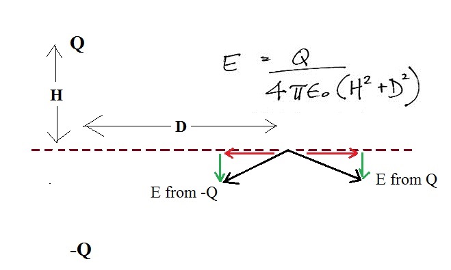
All points on the dashed line (located where the ground
was in the previous picture) have the same potential (zero
potential). You can forget about potential from this
point onwards and can simply write down an expression for
the E field at distance D. There are E fields
produced by Q and also by -Q (the two black vectors in the
figure above). Note the two horizontal components of
the field (in red) cancel. That is what you would
expect at the surface of a conductor. You are left
with two vertical components (green) that add.
You'll need to multiply your expression for E by a sin
Θ or a cos Θ term
to determine the magnitude of the vertical E field
component.
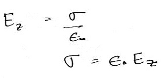
Once you have E as a function of D it is an easy step to
determine the surface charge density σ(D).
Once you have a function for σ(D)
you can multiply it by an increment of area dA and integrate over
the entire surface (from D = 0 to infinity).
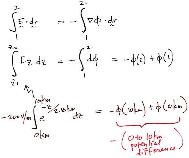
There was less trouble with the second problem. In this case
you were given expressions for the electric field as a function of
altitude and needed to determine the potential difference between
the ground and 30 km altitude. This mostly just means
integrating E. Because you have two expressions for E you
need to integrate from 0 to 10 km and then compute a second
integral from 10 to 30 km. I've set up the integration for
the 0 to 10 km portion below
You need to be careful with negative signs in this question.
I've given many students the option of
redoing portions of Question #1 and/or Question #2 if they
want to.
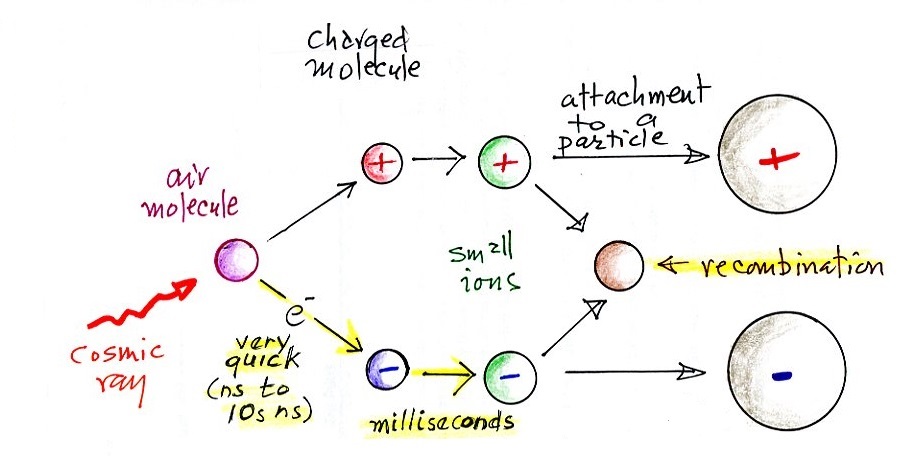
On to the main part of today's class. The lifetime of a
small ion is sketched below. This will serve to introduce
what we'll be covering today.
The first step is ionization of an air molecule. We
discussed the sources of this ionizing radiation in class on
Monday. A cosmic ray is shown in the figure above.
We'll be interested in how long it takes the free electron that is
created in this first step to attach to an oxygen molecule (it
turns out to be very quick, just a few or a few tens of
nanoseconds). Water vapor molecules then cluster around the
charged air molecule to form small ions. This step is also
pretty fast, occurring in milliseconds.
Once created the small ions can recombine. Whatever
results is uncharged. We'll write down an ion balance
equation with a small ion creation term and a recombination loss
term.
Or the small ions can attach to much larger particles in the
air. This lowers their mobility. There charged
particles are known as "large ions." We discuss the
attachment to particles in class on Friday.
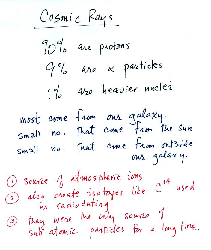
We'll start with some information about cosmic radiation (cosmic
rays). This is the dominant ionization process over the
oceans and over land at altitudes above 1 km.
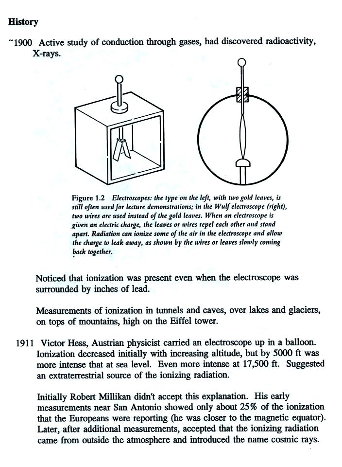
And some historical information (that was on a class
handout). It really was the study of atmospheric
electricity (studies of ionization of air) that lead to the
discovery of cosmic radiation.
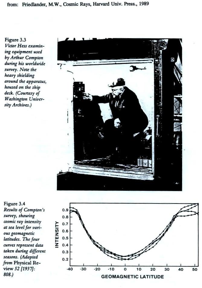
Cosmic ray intensity decreases at the geomagnetic equator
because many of the incoming cosmic rays couple to and
follow the earth's magnetic field lines to the magnetic
poles.
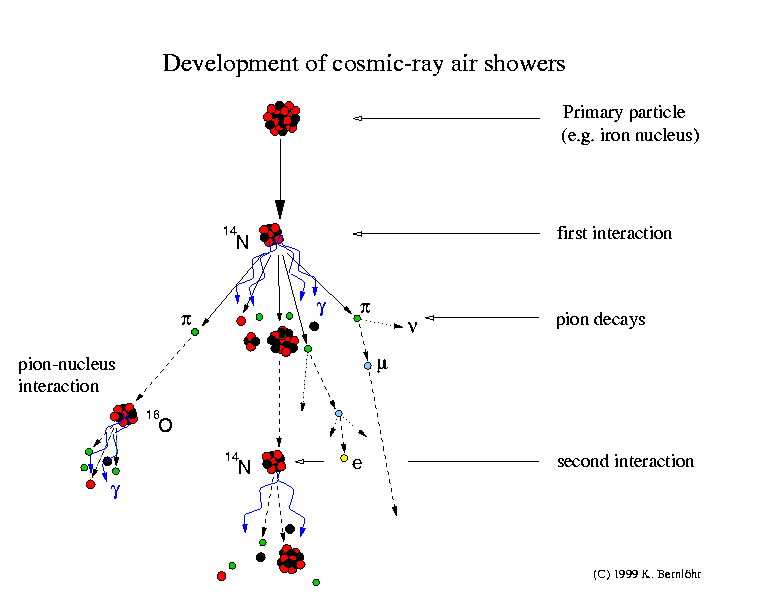
Here is
some information on cosmic ray showers. Very
few of the primary particles reach the
ground. Rather they interact with gas
molecules in the atmosphere and produce a wide
variety of types of secondary particles.
(the figure and text are from: http://www.mpi-hd.mpg.de/hfm/CosmicRay/Showers.html
)
Cosmic-ray
air showers
Cosmic
rays
The earth is
hit by elementary particles and atomic
nuclei of very large energies. Most of
them are protons (hydrogen nuclei) and
all sorts of nuclei up to uranium
(although anything heavier than nickel
is very, very rare). Those are usually
meant when talking aboutcosmic
rays. Other energetic particles in the
cosmos are mainly electrons and
positrons, as well as gamma-rays and
neutrinos.
Interactions
and particle production The
cosmic rays will hardly ever hit the
ground but will collide (interact) with
a nucleus of the air, usually several
ten kilometers high. In such collisions,
many new particles are usually created
and the colliding nuclei evaporate to a
large extent. Most of the new particles
are pi-mesons (pions). Neutral pions
very quickly decay, usually into two
gamma-rays. Charged pions also decay but
after a longer time. Therefore, some of
the pions may collide with yet another
nucleus of the air before decaying,
which would be into a muon and a
neutrino. The fragments of the incoming
nucleus also interact again, also
producing new particles.
The gamma-rays
from the neutral pions may also create new
particles, an electron and a positron, by
the pair-creation process. Electrons and
positrons in turn may produce more
gamma-rays by the bremsstrahlung
mechanism.
Shower
development
The number of
particles starts to increase rapidly as
this shower or cascade of particles moves
downwards in the atmosphere. On their way
and in each interaction the particles
loose energy, however, and eventually will
not be able to create new particles. After
some point, the shower maximum, more
particles are stopped than created and the
number of shower particles declines. Only
a small fraction of the particles usually
comes down to the ground. How many
actually come down depends on the energy
and type of the incident cosmic ray and
the ground altitude (sea or mountain
level). Actual numbers are subject to
large fluctuations.
In fact, from
most cosmic rays nothing comes down at
all. Because the earth is hit by so many
cosmic rays, an area of the size of a hand
is still hit by about one particle per
second. These secondary cosmic rays
constitute about one third of the natural
radioactivity.
When a primary
cosmic ray produces many secondary
particles, we call this an air shower.
When many thousand (sometimes millions or
even billions) of particles arrive at
ground level, perhaps on a mountain, this
is called an extensive air shower (EAS).
Most of these particles will arrive within
some hundred meters from the axis of
motion of the original particle, now the
shower axis. But some particles can be
found even kilometers away. Along the
axis, most particles can be found in a
kind of disk only a few meters thick and
moving almost at the speed of light. This
disk is slightly bent, with particles far
from the axis coming later. The spread or
thickness of the disk also increases with
distance from the axis.
Extensive air
showers with many particles arriving on the
ground can be detected
with different kinds of particle detectors.
In the air the particles may also emit light
by two different processes: Cherenkov light
almost along the shower axis and
fluorescence light in all directions.
Other introductory
material found on the net (HTML format):
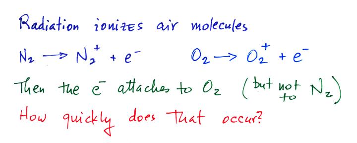
We now know a
little bit more about some of the radiation
sources that ionize air. When neutral oxygen
or nitrogen are ionized you are left with a
positively charged N2or O2
molecule and a free electron.
The electron subsequently attaches to neutral
oxygen molecules (but not to nitrogen). The
time that this takes can be calculated in a
relatively straight forward way. The
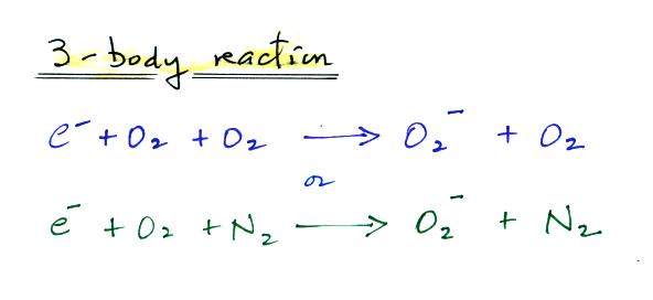
electron attachment is described with a "3-body"
reaction equation.
From what I
learned here,
the electron and two oxygen molecules don't
collide simultaneously. Rather an
electron and an oxygen molecule collide and
produce an "energetically excited reaction
intermediate" which then collides with a
different oxygen molecule that carries off the
excess energy.
The corresponding reaction rate equations are
(the [square brackets] denote
concentration)
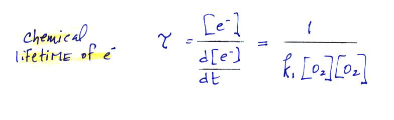
The average
lifetime of a free electron is given by the
following expression
We have the
rate constant k1 but we
also need to know the oxygen concentration in
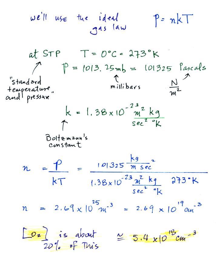
air, [O2].
That's something we can calculate using the
ideal gas law.
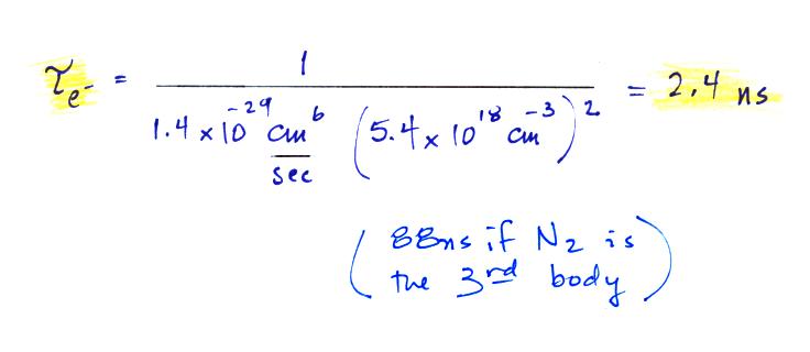
Electron attachment occurs very quickly, in
a few or a few 10s of nanoseconds.
The
attachment time is very short when the
oxygen and nitrogen concentrations are
high. The time gets longer higher in
the atmosphere where [O2] and
[N2]
are lower.
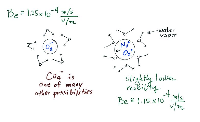
The next step in small ion formation is
clustering of a chemical species of some
kind around the positively and negatively
charged ions. This
occurs on a millisecond time scale.
In the figure above we show ionized
nitrogen and oxygen molecules. This
is just one possibility. CO4-
is
apparently
one
of
the
more
common
ions found in the centers of these
molecular clusters also. And
something other than water may envelope
the central ion.
The mobilities of positively and
negatively charged small ions are slightly
different. Typical values are shown
above. The positively charged small
ions have a slightly higher mobility
(slightly lower drift speed) than the
negatively charged ions.
What happens to the small ions once
they are created? How long do they
survive? For that we need an ion
balance equation.
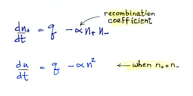
The concentration of small ions (the
positively charged ions are considered in
the first equation) will depend on the ion
production rate, q, and the rate at which
ions recombine and neutralize each
other. Because the free electrons
attach to oxygen molecules so rapidly and
the clustering of water vapor molecules
around charged molecules is also quick
they don't slow down the formation of
small ions. The key step in the
formation of small ions is the rate of
ionization.
A simpler version of the equation (the
bottom equation above) can be written if
we assume that the concentrations of
positive and negative small ions are
equal.
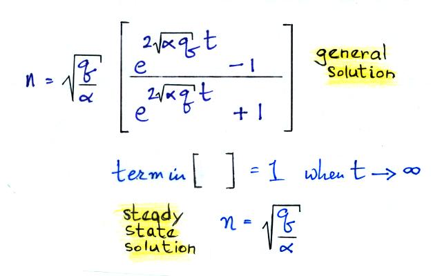
The next figure gives the general and
steady state solutions to the ion balance
equation.
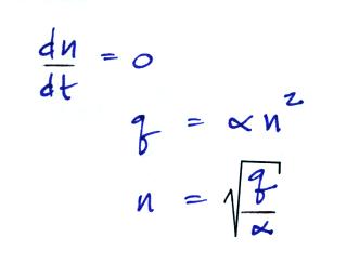
We get the steady state concentration as t
goes to infinity. At steady state,
dn/dt is zero so here's a shorter, easier
way of detemining the steady state
solution.
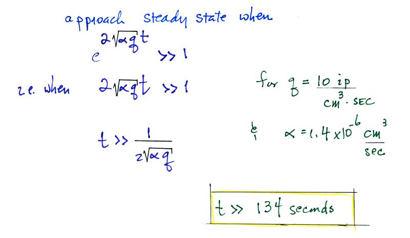
How
long does it take to get to steady
state?
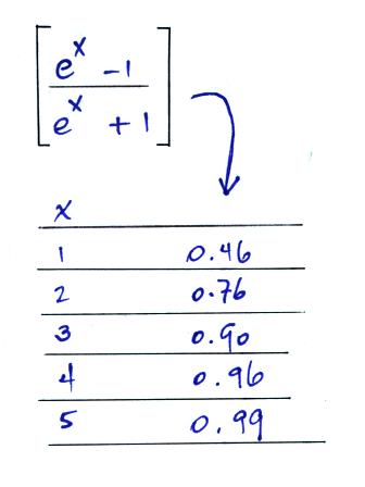
The 2√(αq) t
term doesn't really need to be very
big before you start to approach
steady state.
.
You get to
steady state pretty quickly (~10
minutes). We're really not
going to be looking at fair
weather phenomena that happen more
quickly than that.
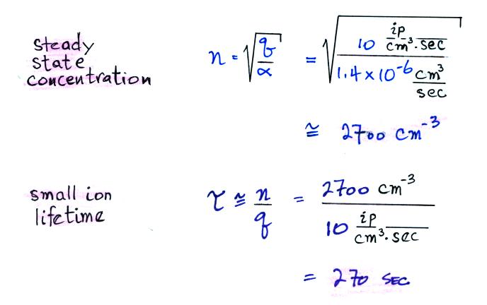
Next
we can calculate the steady state
concentration and then the lifetime of
a typical small ion (concentration
divided by production rate or by
recombination rate since they are
equal at steady state)
Remember
that n is the concentration of either
the positive or negative small ions
(which we have assumed have equal
concentrations).
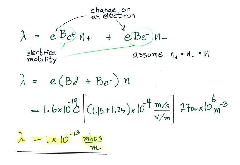
We can also estimate the conductivity
(remembering that both positive and
negative small ions contribute to the
conductivity and taking into account
that the positive and negative small
ions have slightly different
electrical mobilities). We
assume that the small ions carry a
single electronic charge.
This
seems a little high (maybe 5 times
higher than values we've been using in
class and on homework
assignments). But this is a case
where there are just small ions and no
particles. We'll look at the
effects of particles in class on
Friday. Particles are an
additional small ion loss process and
we would expect that to lower the
equilibrium concentration of small
ions. That will also reduce the
conductitivy.

 .
.