Monday Feb. 2, 2015
The first homework assignment was collected today. Once I
have all the assignments in hand I'll try to post some answers
online. I'll also try to get the graded papers back to you
this week.
A couple of E field related topics to finish before we get into a
section on currents and conduction of electricity in the
atmosphere.
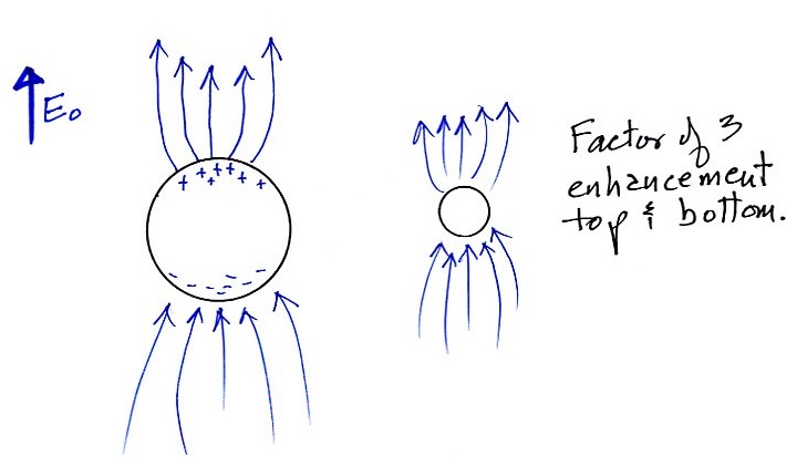
The "conducting sphere in a uniform electric field" problem
that we worked out last in class Friday revealed that the electric
field will be enhanced by a factor of 3 at the top and bottom of
the sphere (assuming the field is vertically oriented). This
3 times enhancement does not depend on the diameter of the sphere.
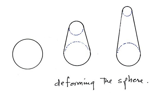
What if we were to stretch the sphere vertically in such a way
that one part ends up with more of a point than the other.
It would be very hard to determine the field enhancement of an
object like this analytically. I'm sure there are ways of
determining the enhancement numerically.
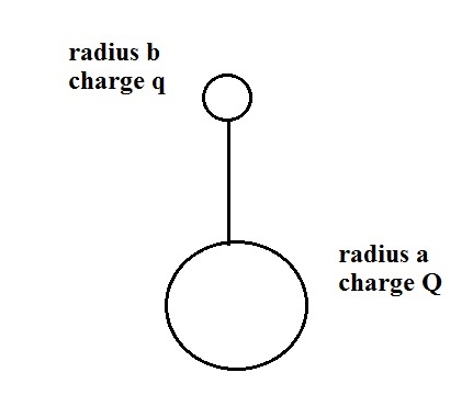
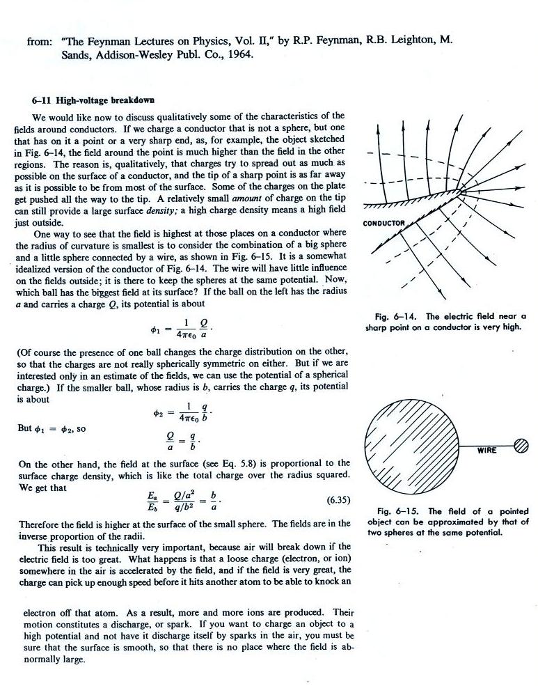
To get some feeling for how the field enhancement at the top
and bottom of an object like this would differ, Richard Feynman
considers two separate spheres with different radii and then
connects them with a wire so they are at the same potential.
I've reproduced his discussion below:
This might require a little
explanation (I had a little trouble the first time I read it)
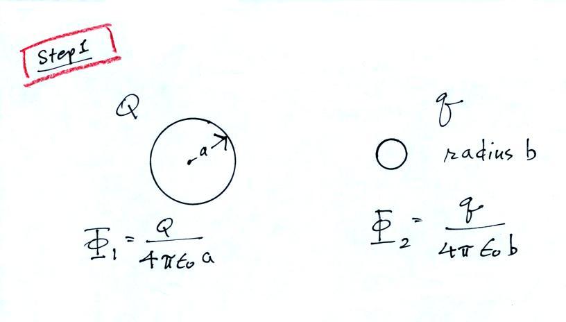
In the first step we consider
two unconnected spheres and write down the potential at the
surface of each
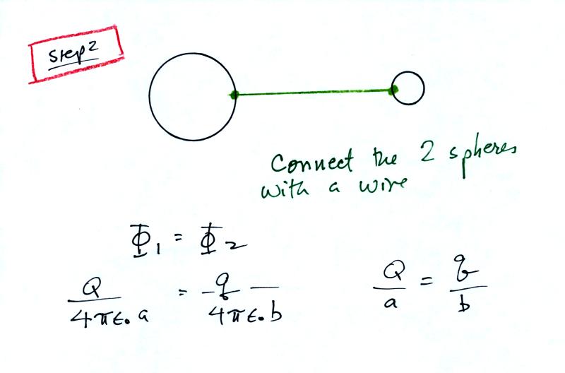
Then you connect the two spheres
with a wire which forces the two potentials to be equal (this
would of course cause the charge to rearrange themselves and
turn this into a much more complex problem, but we will ignore
that).
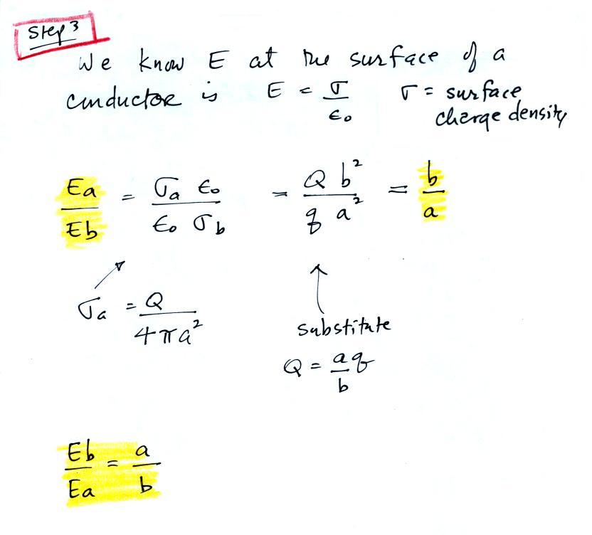
Finally we write down
expressions for the relative strengths of the electric fields at
the surfaces of the two spheres (we assume Q and q would be
uniformly spread out over the two spheres which wouldn't be
true). We see that the field at the surface of the smaller
sphere is a/b times larger than the field at the surface of the
bigger sphere. Since a > b, the field above the smaller
sphere is enhanced.
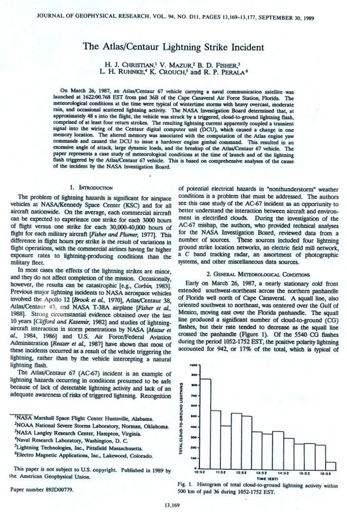
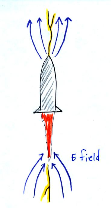
Here is a real example of field enhancement
that lead to triggering of a lightning strike and subsequent
loss of a launch vehicle (you'll find the entire article here)
In this case the rocket body together with
the exhaust plume created a long pointed conducting
object. Enhanced fields at the top and bottom triggered
the lightning discharge. Note the branches point away from
the rocket. This indicates that the leader process at the
beginning of the discharge started at the object and moved
outward.
Lightning also strikes aircraft. Here's an
example. Often, probably usually, the discharge is
initiated by the airplane.
We'll talk about rocket triggered lightning later in the
course. I'm referring to lightning that is purposely
triggered so that it can strike instrumentation on the ground
and studied at close range.
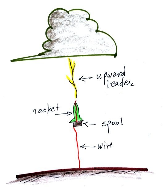
Here's an
example from the ICLRT (International Center for Lightning
Research and Testing) operated by the University of
Florida.
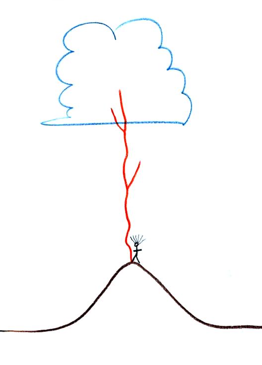
Enhancement of the E field at the top of a
mountain (or tall building or structure) is sometimes high
enough to trigger lightning also.
Note the direction of the branching. This indicates that
this discharge began with a leader process that traveled upward
from the mountain. Most cloud to ground lightning discharges
begin with a leader that propagates from the cloud downward toward
the ground. We will of course look at the events that occur
during lightning discharges in a lot more detail later in the
semester. Here are some
examples filmed in Germany (probably developing off tall
towers of some kind, perhaps wind turbines) and strikes to
the Empire State Building.
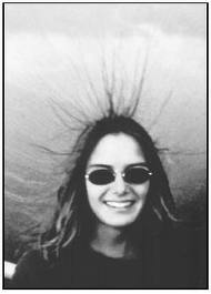
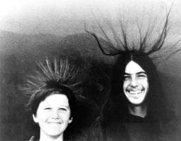
The E fields on mountain tops under a thunderstorm can be strong
enough to lift a person's hair as illustrated below. This is
a dangerous situation to be in
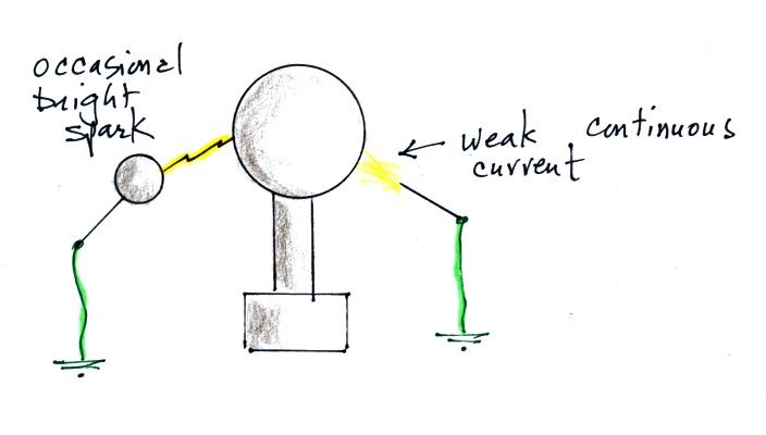
And finally the ability of a point to draw off or throw off
electrical charged that so interested Benjamin Franklin involves
enhancement of the E field.
A pointed conductor brought near a Van de Graaff generator
enhances the field enough to ionize air, create charge carriers,
and make the air more conducting. A weak current flows
between the Van de Graaff and the point. Charge on the
generator is not able to build to the point where a large bright
spark occurs.
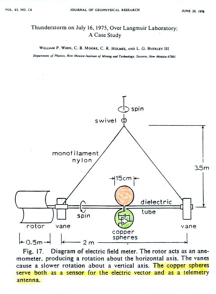
Here's an example of a very cleverly designed
instrument that has been used to measure electric fields above
the ground and inside thunderstorms (you can download the
complete Winn et al. 1978 publication here).
Two metal spheres are attached to and spin
vertically around a horizontal shaft (the shaft also spins
azimuthally). The instrument is launched under a
thunderstorm and is carried upward by balloon.
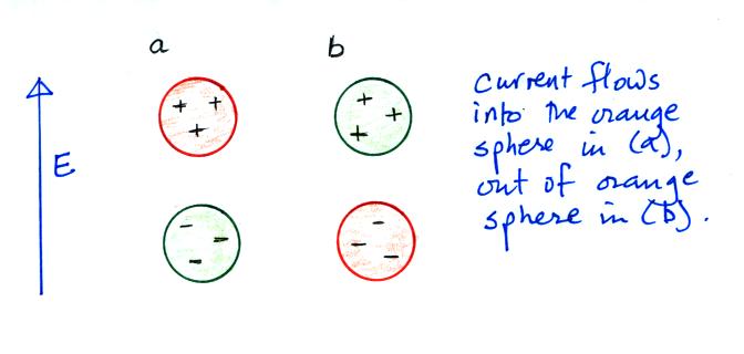
As the spheres spin, a current will move back
and forth between them. The amplitude of the current will
depend on the charge induced on the spheres by the electric
field. The induced charge will, in turn, depend on the
intensity of the E field.
Determining how the two conducting spheres will enhance the
electric field is a more complex problem than we considered in
the last lecture but it has been worked out analytically (don't
worry we won't be looking at the details). You could also
work it out numerically or determine the enhancement
experimentally. Note that the two spheres also act an
antenna for transmitting data back to the ground.
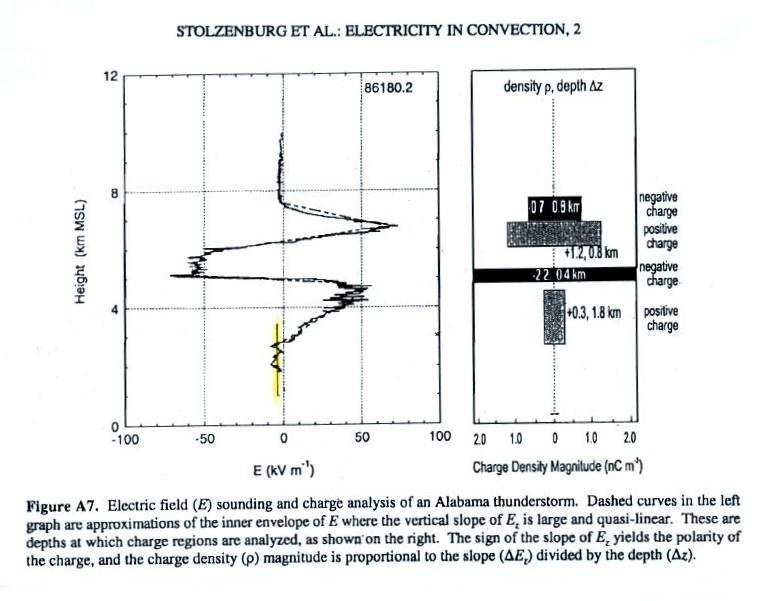
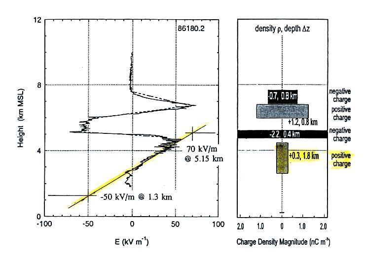
The next figure shows an example of data obtained with an
instrument like this (it is from a different publication which
you can download here,
but a similar instrument was used).
We're going to take a more careful look at 2 parts of the E
field plot. First the small highlighted portion at the
bottom of the plot. Here the sensor was below the lowest
charge layer in the cloud (perhaps even below the base of the
cloud) and the E field seems to be fairly constant varying between
about -2 and -4 kV/m. At first glance that seemed
surprising; I would have expected to see the field increasing as
the balloon and its sensor got nearer the charge.
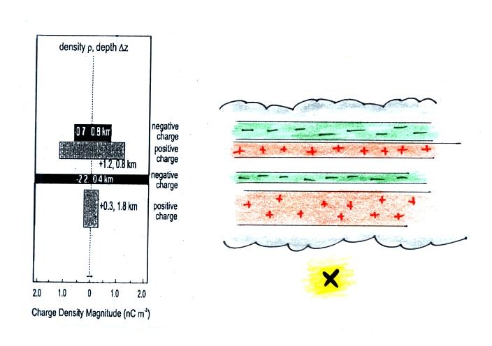
Can we use the charge density information at right in the figure
to explain this field?
There are 4 layers of charge. The field at Pt. X below
the lowest layer will be a superposition of the fields from each
of the layers above. We'll assume each of the layers
is of infinite horizontal extent (sort of a 2-D version of the
infinite uniform line of charge). We can use the integral
form of Gauss' Law to determine the field above and below a layer
of charge.
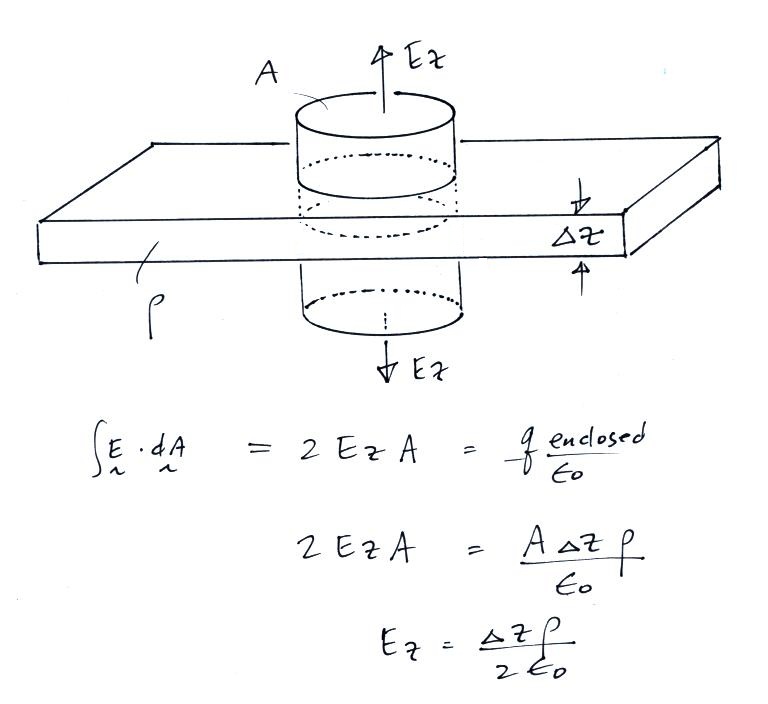
I think you can argue "by inspection" that the field above and
below the infinite layer of charge will have just a
z-component. Also because the layer is of infinite extent
the field strength will be the same at any distance above or below
the layer.
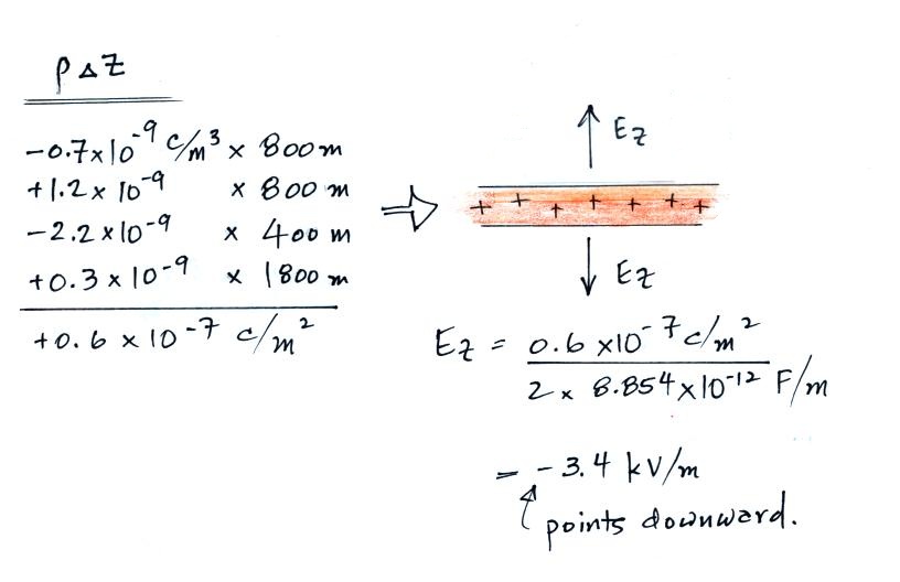
So we compute ρ Δz for each of the layers, add the results
together and use that to compute the field using the equation
above.
Below the cloud we find that the field is negative (points
downward) and has an amplitude of 3.4 kV/m. This agrees very
well with what is shown in the E field sounding.
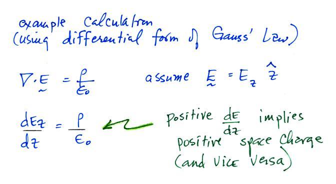
Next we'll examine the increasing E field as the sensor
passes through the lowest layer of charge.
The E field change appears linear and we can measure the slope of
the field change and the differential form of Gauss' Law to
determine the volume space charge density.
Note that dE/dz is positive on the E field sounding between about
2.7 km and 4.5 km or so. This coincides with a 1.8 km thick
layer of positive space charge. The slope turns negative
between about 4.7 km and 5.1 km where there is a layer of negative
charge. The E field reaches a peak positive value at about
4.6 km, a point that is in between the layers of positive and
negative charge.
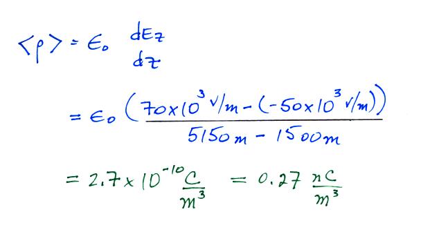
We can determine the slope of the line highlighted in yellow and
use that to determine the average volume space charge density in
the layer of positive charge.
The value we obtain (0.27 nC/m3)
is in good agreement with the 0.3 nC/m3 value
given in the paper.