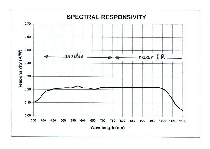
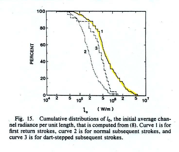
Next we will look at a couple of examples
of a completely different type of ground based optical
measurement. The figure below at left is from adapted
from Jordan
and Uman (1983) and shows how light signals
coming from narrow vertical segments of a lightning channel
from a natural subsequent return stroke might vary with
altitude. The signals were recorded on
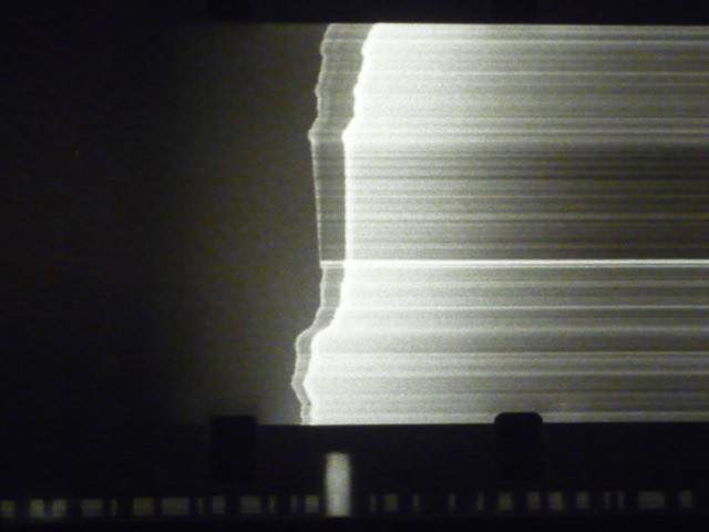
film with a high speed streaking camera like has been used to
measure return stroke velocity. A example of a streaking
photograph from an entirely different event is shown at right
(photo credit: Dr. Vince Idone, State Univ. of NY at
Albany). The image recorded on film was then
digitized. The figure at left actually shows
film density versus altitude (the film density values were
roughly proportional to the logarithm of light intensity).
The streaking camera shutter was triggered (opened) by the
first return in a flash and remained open for 0.5
seconds. Only subsequent stroke signals were captured on
film
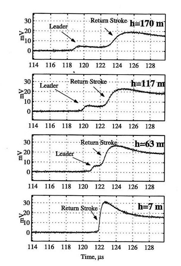
The downward propagating dart leader can be seen clearly on
the 37 m and 78 m records. The upward propagating return
stroke can be see on all 9 records. Jordan and Uman
reported that the amplitude of the return stroke fast initial
peak decays exponentially with altitude with a decay constant
of 0.6 to 0.8 km. The relatively constant amplitude
portion of the signal following the fast peak is relatively
constant between the ground and cloud base.
Changing light signals like these suggest that the return
stroke current waveform also probably changes shape with
increasing altitude (though Jordan and Uman suggest that the
current decays much more slowly than the light signals).
You may remember that the transmission line model assumes that
the return stroke current remains constant with increasing
altitude.
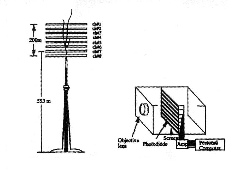
Wang
et al. (1995) describe a more modern system that they
first used to study lightning striking the CN Tower in Toronto
(the 3rd tallest building in the world).
(
source
of this image)
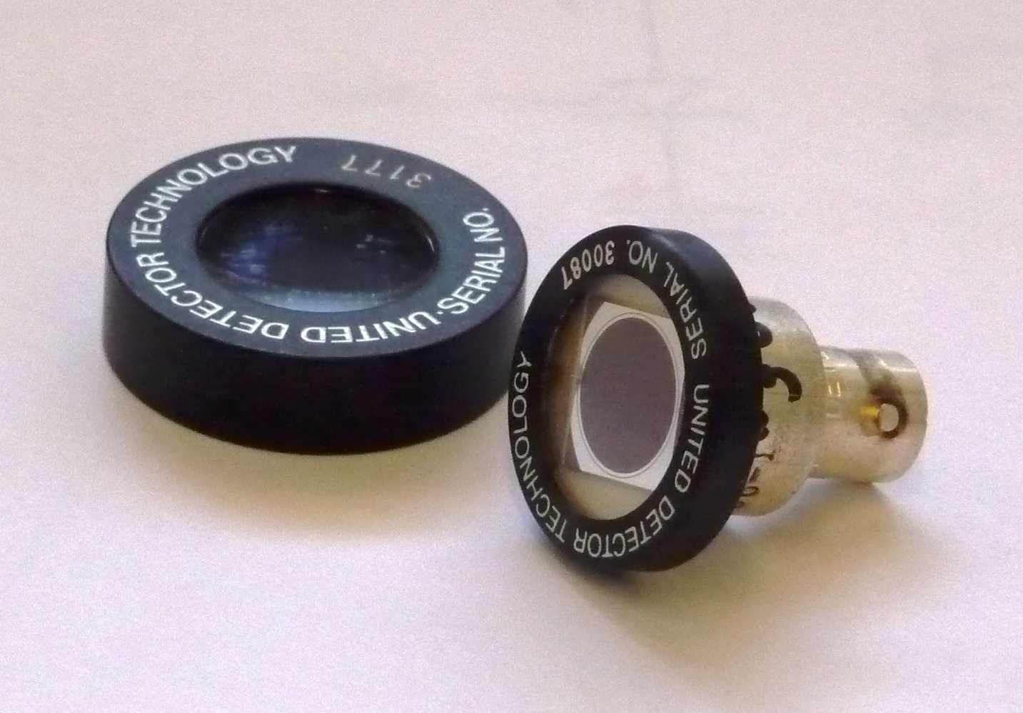
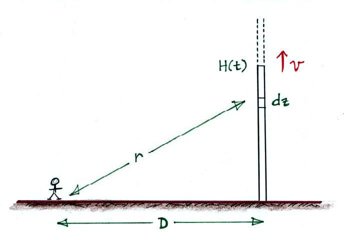
Their sensor is shown below at
right.
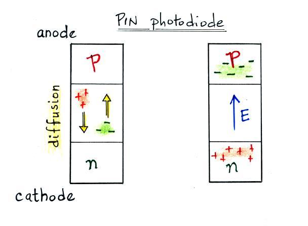
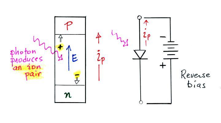
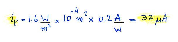
Eight rectangular photodiodes (1 mm x 24 mm) are mounted in
the focal plane of a camera lens. The photodiode signals
are amplified and connected to a multi-channel 8 bit digitizer
( 0.2 us sample interval and 200 us duration record with 10 ns
synchronization between signals). Waveforms were stored
on a computer. The sensor was placed on the roof of a
building located 1.8 km away from the CN Tower. A
roughly 200 m x 200 m area above the tower was imaged (the
lowest channel, ch#8, was actually positioned below the top of
the top because lightning sometimes strikes below the tallest
point on the tower).
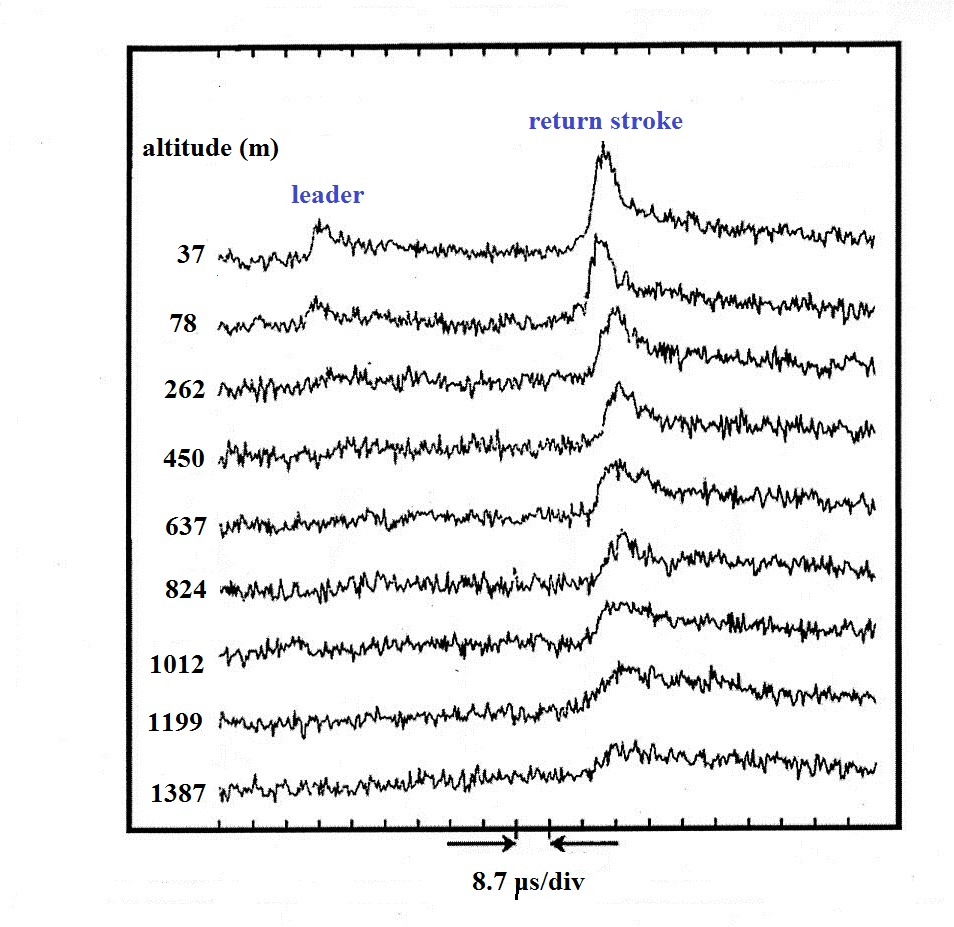
An example of data from a normal dart leader - subsequent
return stroke discharge are shown below (adapted from the Wang
et al. paper).
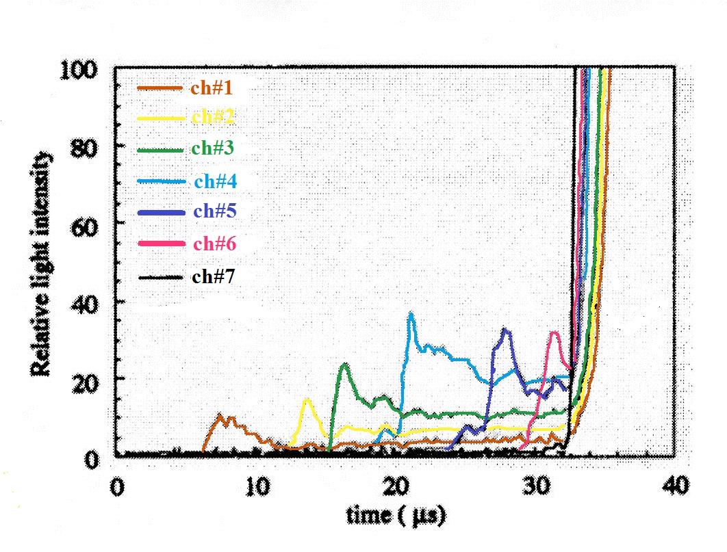
You can clearly see the downward
propagating dart leader on the top 3 records followed by an
upward propagating subsequent stroke. This the first
subsequent stroke in a 7 stroke triggered lightning
flash. The stroke had a peak current of 28 kA. The
4 channel photodiode sensor was about 300 m from the strike
point; the light signals above come from roughly a 1 m
vertical segment of the channel. Note the significant
change in the shape of the return stroke front in just the
first 170 m above the strike point.
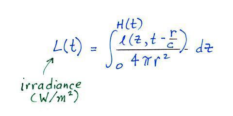
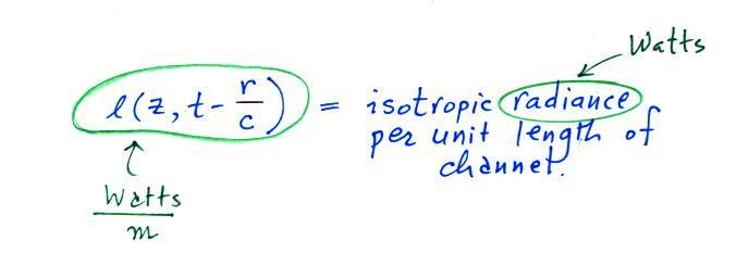
Measurable time delays from signals from know altitudes can be
used to determine both leader and return stroke
velocities. Some additional discussion of that
will be added.