Today we will be looking at satellite detection and location of
lightning. We'll just look at a couple of recent
satellite sensors, the Optical Transient
Detector (OTD) and the Lightning Imaging
Sensor (LIS), that detect the optical emissions of
lightning during the day and at night from low earth orbit.
Both were designed and built by researchers at the NASA Marshall
Space Flight Center. A new and improved lightning mapping
sensor will be on the GOES-R
satellite scheduled to be launched in 2015 (you can read more
about the Geostationary Lightning Mapper [GLM] that will be about
GOES-R here
and here
).
Here's a list of some of the areas where regional or
global satellite observations of lightning might be of interest
(from Christian
et al., (1989) and the GLM site above).
magnetospheric and ionospheric research
atmospheric chemistry
nitrogen fixation
ozone reactions and stratospheric chemistry
storm physics
lightning activity/storm intensity
ocean/land lightning ratio
hurricane electrification
lightning/tornado activity
lightning/precipitation
initial electrification
identifying and locating deep convection
initialization of weather forecast models
climate studies
ground and aviation hazard warning
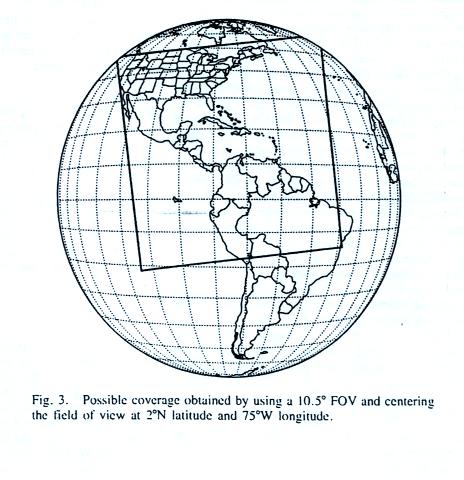
This figure provides an idea of the area viewed by a lightning
mapper aboard a satellite in geostationary orbit. We will
see that most lightning activity falls between 35 S and 35 N
latitude. The GLM will be aboard both GOES East and West
satellites and will cover a much larger region than shown here (ref). Christian
et al. (1989) contains a detailed discussion of the factors
that must be considered in the design of a satellite lightning
sensor (and lists some of the earlier satellite observations of
lightning). Prior to designing the OTD and LIS, the NASA
Marshall group also made extensive measurements of lightning
optical emissions from a platform on a high-altitude aircraft
flying well above the tops of thunderclouds (a U-2 aircraft flying
at approximately 20 km altitude).
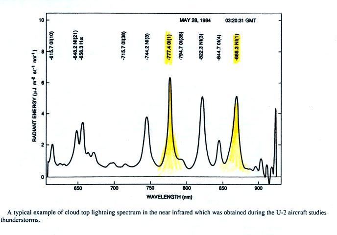
An example of a lightning spectrum recorded by the U-2 aircraft
is shown below (from Christian et al. 1989).
The U-2 measurements did indeed show that both cloud to ground and
intracloud discharges could be detected from above cloud top
(determining the type of discharge process using the optical
signals is an area of current research). The 777.4 nm and
886.3 nm features (OI and NI) highlighted above each contain 5 to
10% of the optical energy in a lightning flash. The 777.4 nm
OI(1) line was ultimately chosen for the satellite detectors.
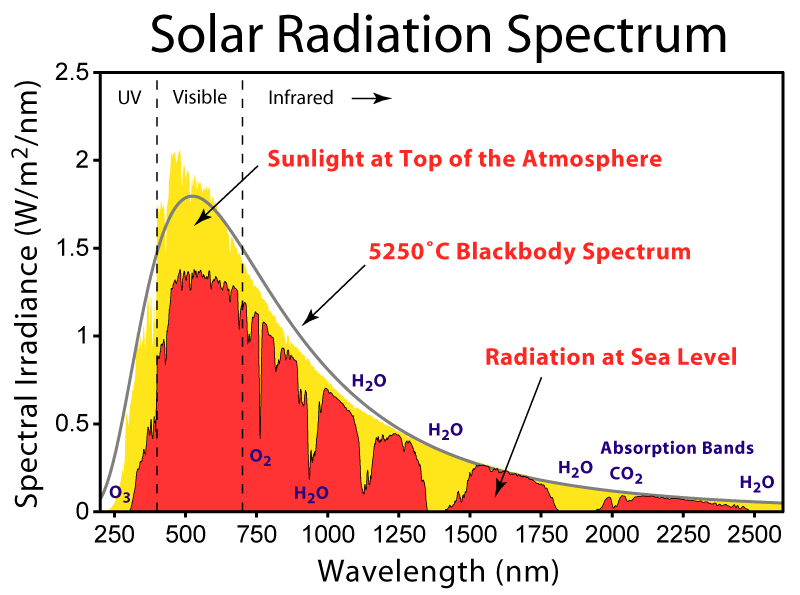
Some of the early satellite observations of lightning were made
only at night. The OTD, LIS, and GLM will observe lightning
during the day and at night. Lightning occurs in clouds and
clouds are very good reflectors of the visible and near IR
wavelengths in sunlight. Steps must be taken to distinguish
or separate the relatively weak lightning signal from the brighter
reflected sunlight. The solar spectrum as would be observed
at the top and bottom of the atmosphere is shown below (source).
The spectrum of reflected sunlight might
differ somewhat.
We should take a quick look at the shape of the optical signals
produced by lightning discharges. And because the lightning
will be viewed from above the thunderstorm top we need to look at
the effects that scattering by cloud particles will have on the
light impulses.
Here's a portion of a larger lecture on ground based
measurements of lightning optical signals (and what can be learned
from them)
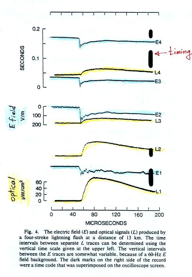
Examples of recorded fast electric fields (E, shaded blue) and
associated optical signals (O, highlighted in yellow) are shown
below (from Guo
and Krider, 1982).
This was a
four stroke cloud-to-ground discharge that occurred at 13 km
range. The first return stroke is shown at the bottom of
the figure. The first 50 μs or so of the record is the
stepped leader. This is followed by an abrupt rise to
peak. Notice that the E field signal is still increasing
in amplitude at the end of the record. This indicates
some of the electrostatic field component is present which is
typical of a return stroke field recorded at a range of about
10 km. These waveforms were photographed on moving
film. The dark black timing marks were from an LED that
would flash on and off to code the absolute time onto the
film.
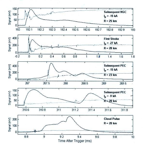
And a more recent example (Quick
and Krider, 2013), recorded with modern waveform
digitizing equipment is shown below
Signals from a first return stroke, subsequent return strokes
(NGC is a channel with a new ground contact point, PEC a
pre-existing channel), and a cloud discharge are shown. Note
the time scales are in milliseconds. The large divisions on
the time scales range from 100 to 500 microseconds.
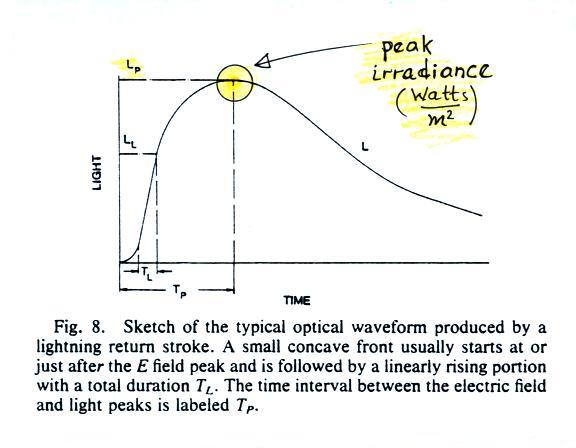
A typical return stroke optical signal. We can use a
measurement of the peak optical signal amplitude (in volts) to
determine the peak irradiance, Lp
(in W/m2). Then if the
range to the discharge is known we can estimate the peak optical
power output, P (in Watts) from the return stroke. This is a
variable that would be need to be known when designing a satellite
detector.
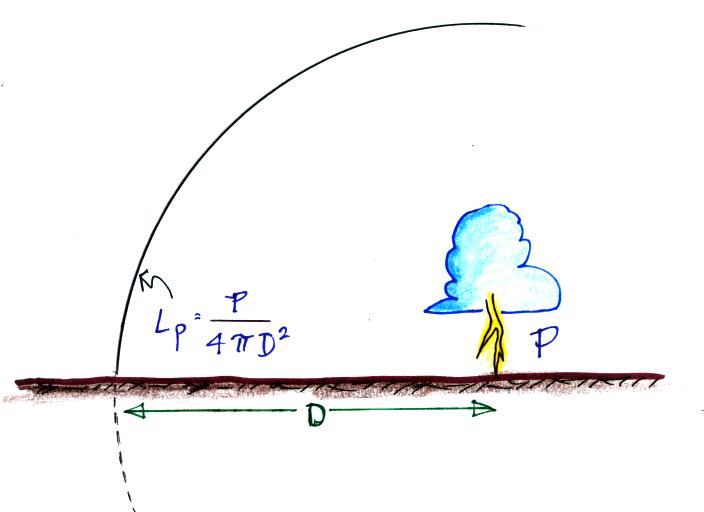
We treat the lightning discharge as a point source and assume the
optical power output during the strike will expand evenly outward
in a sphere. We measure the peak irradiance, Lp, a distance D from the source
(W/m2 on the surface of the
expanding sphere). So to estimate P we simply multiply the
measured values of Lp by the
area of the sphere.
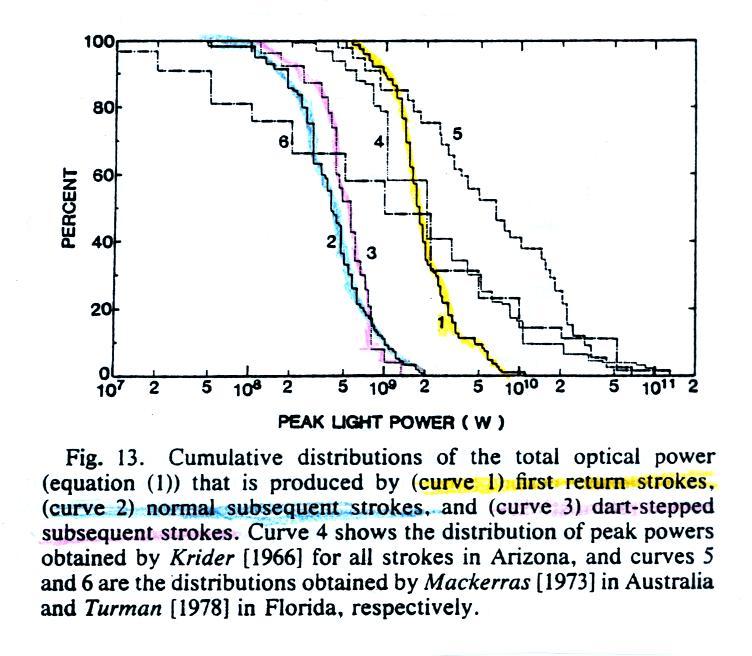
Cumulative distribution of peak optical power estimates. 50%
of 1st return strokes have a peak optical power output of about 2
x 109 Watts or more.
Peak power emitted by subsequent strokes is almost a factor of 10
less.
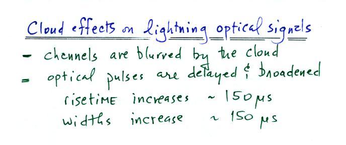
The relatively fast signals shown above will be broadened while
traveling upward through the thunderstorm cloud
Just like frosted glass, clouds will blur any image of the
lightning channel inside the cloud. The optical signal
risetime and pulse width are each increased by about 150
microseconds. The following figure helps to understand why
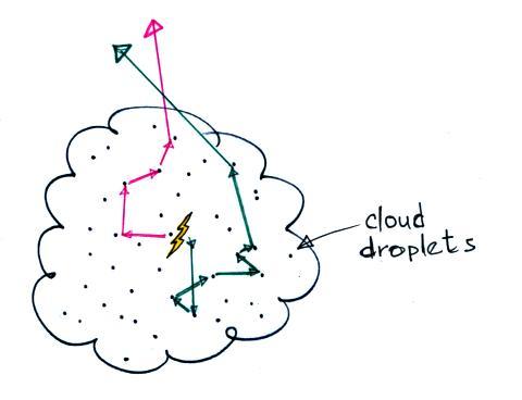
this is true.
Photons emitted by a lightning
channel are scattered (redirected) multiple times before
leaving the cloud. The path in pink undergoes a
relatively low number of scatters. The green path is
scattered more times and takes longer to escape from the
cloud. It is difficult to distinguish between
cloud-to-ground and intracloud discharges.
Somewhat surprisingly perhaps, there is very little
absorption of the light signal by the cloud.
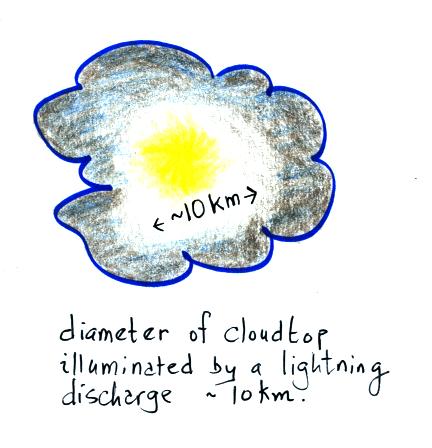
A lightning flash illuminates about 10 km diameter of the
cloud top. Ideally this would just fill a single pixel
on the CCD satellite detector.
We'll spent most of the remainder of our discussion on the
Optical Transient Detector (OTD). This is the first of two
satellite "lightning mappers" designed by the people at the NASA
Marshall Space Flight Center. You can read more about that
research group and some of the activities on the Global Hydrology
and Climate Center webpage.
The OTD was a prototype for the Lightning Imaging Sensor.
The OTD was launched on Apr. 3, 1995 and turned off in Mar. 2000,
having operated 2 years beyond its expected lifetime.
It was launched into a nearly circular orbit 740 km (~450 miles)
high. The orbit was inclined 70o (relative to the Equator) so the satellite
coverage extended from 75o S
to 75o N latitude.
For comparison the GOES GLM will be launched into geostationary
orbit and will have coverage extending from 52o S to 52o N latitude.
The OTD field of view was about 1300 km x 1300 km (about 1/300
th of the earth's surface) and was imaged onto a 128 pixel x 128
pixel CCD sensor array (thus about 10 km x 10 km per pixel which
is about the size of the cloud top illuminated by lightning)
Location accuracy (at nadir) was about 8 km.
The orbit precesses about 15 minutes (1/4 of a degree) per
day. It takes about 50 days for the satellite to review a
specific location on the earth's surface at the same time of
day. The GOES GLM will view the same scene continuousy.
In a year the OTD images most locations for a total time of >
14 hours (400 individual over passes).
The OTD detects lightning during the day and at night. The
typical daylight cloud background (sunlight reflected off the
cloud tops) is 50 to 100 time brighter than lightning.
Several steps must be taken in order to detect lightning signals
superimposed on this bright background.
(i) The pixel size corresponds roughly to the size of
the cloud top illuminated by lightning (maximize the signal to
background noise)
(ii) A 1 nm narrow band interference filter centered on the
777.4 nm OI emission was used. Much of the reflected
sunlight background falls at other wavelengths and was
blocked. The same feature will be used in the GOES GLM
(iii) CCD signals were integrated for 2 ms - well over the
duration of the lightning optical pulse. The same
integration time will be used in the GLM.
(iv) successive frames were subtracted. This subtracts out
much of the slowly time varying background signal
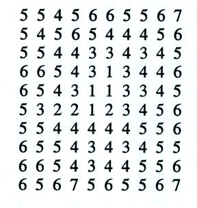
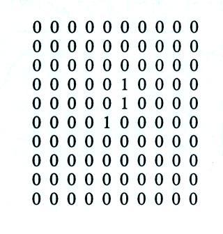
This last process is illustrated below
The leftmost image shows a picture of the scene. The middle
two frames show the CCD data for pictures taken of the scene with
and without a lightning. It's hard to see the lightning
until you difference these middle images. The lightning
appears in the 4th picture (the three pixels with values of 1 in
the middle of the scene).
There are still sources of noise such as sun glint that create
erroneous lightning counts. The South Atlantic Anamoly is
also a source of false triggers. This is a region where the
Van Allen Radiation Belts make their closest approach to the
earth's surface. The inner belt contains mainly high energy
protons. When the satellite passes through the belt, the
high energy particles strike the CCD array and produce anamolous
triggers.
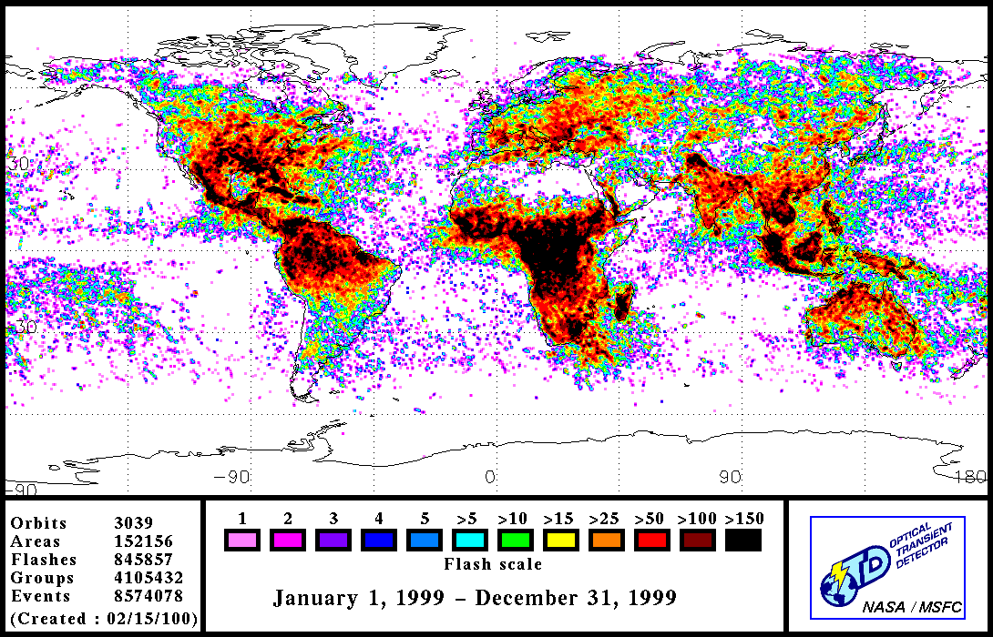
Here are some images of lightning activity derived from OTD
data.
This image shows all of the lightning detected in 1999.
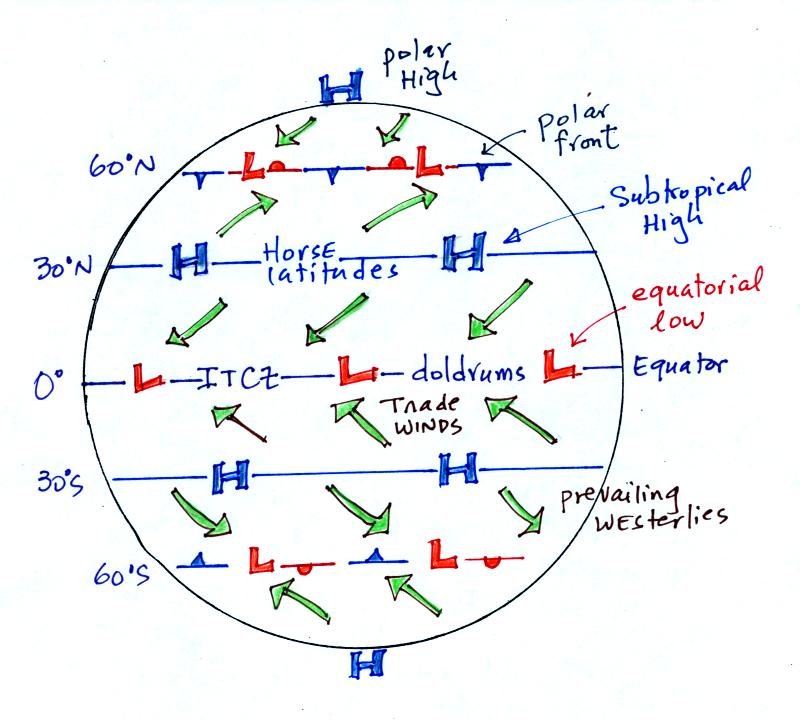
Most of the lightning detected is found over land affected by the
Intertropical Convergence Zone (ITCZ). This refers to a
feature in the 3-cell model of the earth's global
scale
circulation pattern.
The figure above shows most of the surface features (high and low
pressure belts and winds) predicted by the 3-cell model. The
ITCZ is nominally located near the Equator (also labelled the
equatorial low in the figure above). Surface winds converge
and produce rising air motions. Since
this equatorial air is often quite moist you can often see a
band of clouds at or near the equator on a satellite
photograph (if that link doesn't work try this
one). The ITCZ will
move north of the Equator in summer (northern hemisphere summer)
and south of the equator in the winter.
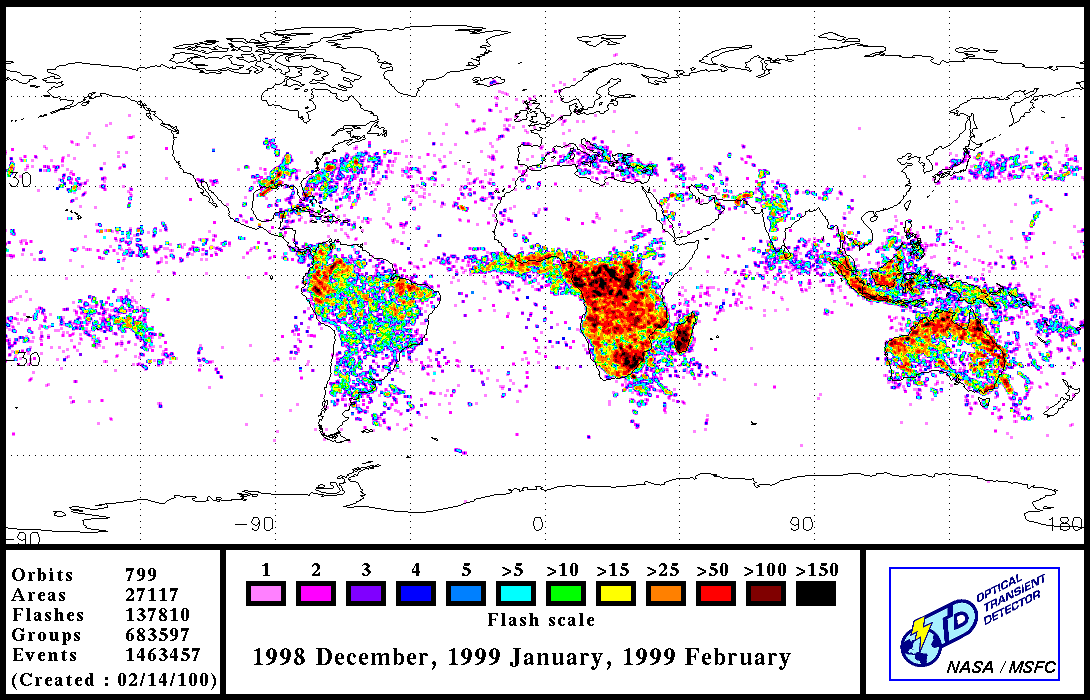
Here's the lightning detected during the months of December,
January, and February 1999. Note how the activity has
shifted into the southern hemisphere. The activity at higher
latitudes in the northern hemisphere might be associated with
storms forming along the polar front.
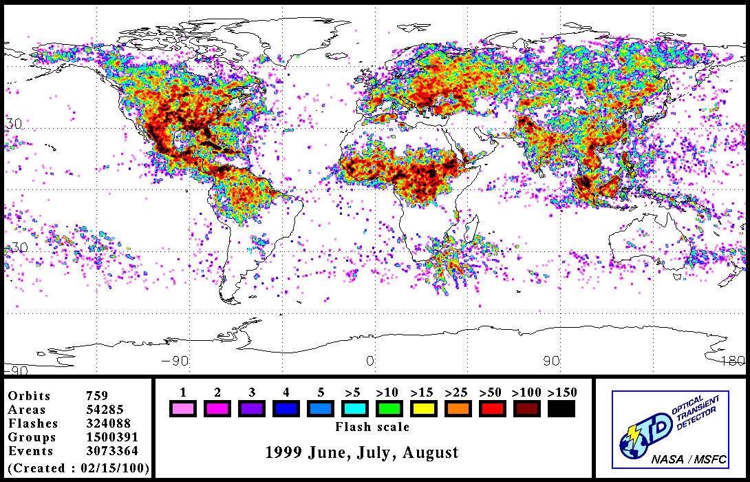
This is the June, July and August map for the same year.
Activity is now primarily in the northern hemisphere.
78% of the lightning detected (and remember the OTD doesn't
distinguish between cloud-to-ground and intracloud discharges) is
found between 30 S and 30 N latitude. 88% of the lightning
is found over continents, islands, and coastal regions.
There is much less activity over the oceans.
One interesting result from 5 years of OTD lightning data is a
new estimate for the global lightning flashing frequency:
44 flashes/sec
(plus or minus 5 flashes/sec)
This is about half of the 100
flashes/sec value that was long thought to be true. The
100 flashes/sec value dates back to about 1925.
You can view a more up to date global lightning image from
the Lightning Imaging Sensor (LIS) here.
This was the 2nd prototype sensor developed by the NASA
Marshall Space Flight Center group. The LIS
was launched in November, 1997 and is still operating.
It detects and locates lightning between 35o S to 35o N
