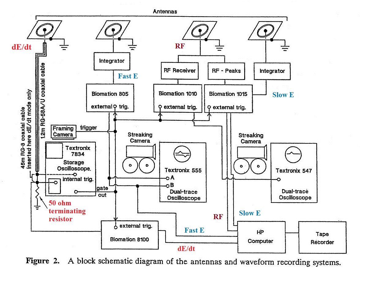
You should recognize the flat plate E field
antennas shown at the top of the figure. Separate
antennas were used for dE/dt, Fast E, a 5 MHz RF signal, and a
Slow E signal. The signal cables from the Fast E and
Slow E antennas were connected to integrators. We
discussed all of this earlier in the semester so that should
be familiar.
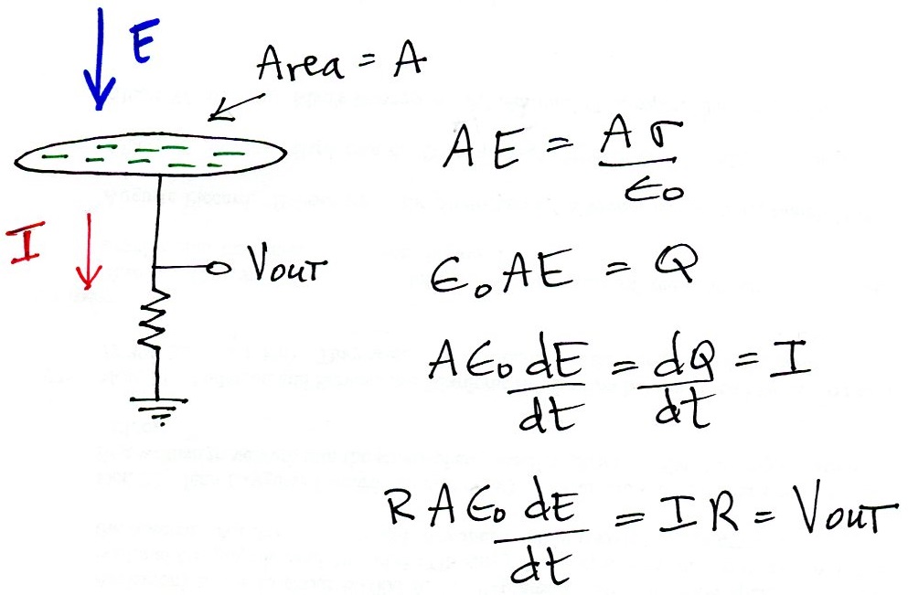
For dE/dt, the cable from the flat plate antenna (the left most antenna above) was not connected to an integrator. Rather it was connected to a 50 ohm resistor, the characteristic impedance of the coaxial cable. The voltage that appears across this resistor is proportional to dE/dt as shown below.
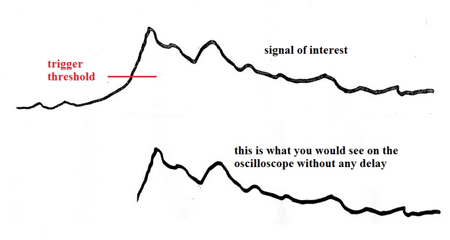
Note the dE/dt signal cable is here shown connected to the internal trigger of the storage oscilloscope (the 5 MHz RF signal was also used to trigger the storage oscilloscope). The dE/dt signal then ran through a 45 m length of coaxial cable before being connected to the input of the storage oscilloscope. The 45 m length of cable acted as a delay line (about 150 ns of delay). The hope was that with sufficient "pretrigger" signal you could establish an accurate zero. The figure below shows an oscilloscope display of a signal with and without delay.
The oscilloscope begins to sweep when the signal crosses the trigger threshold. Without delay you would only capture a portion of the rise to peak (left figure). With sufficient delay (right figure) you could capture the entire front edge of the signal.
Some examples of dE/dt signals recorded with a system like the one above are shown below at left. An E signal obtained by integrating the dE/dt waveforms is shown at right. LS and RS indicate leader step and return stroke signals respectively.
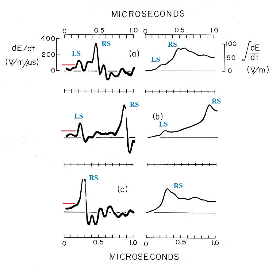
The dE/dt signals were recorded on a very fast time base. A storage oscilloscope was oscilloscope signal if a storage scope hadn't been used. The red line shown at the left of each of the dE/dt signals shows the approximate storage oscilloscope trigger level.
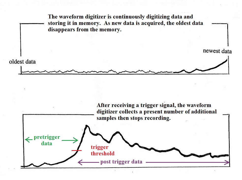
It is much easier to obtain pretrigger signal when using a
waveform digitizer. A waveform digitizer continuously
digitizes the incoming signal. It doesn't attempt to
store all of this data only the most recent samples. As
new data is acquired and added to the memory, the oldest data
is pushed out of the memory. Once a trigger signal is
received, the digitizer collects a preset number of additional
samples and then stops recording. The data in memory is
preserved until it can be read or displayed (both were done in
the system above).
As best I can remember the waveform digitizers above had the following characteristics
The Traveling Current Source lightning return stroke current model
You may remember in the experimental test of the transmission line model that simultaneous measurements of Epeak and Ipeak and also (dE/dt)peak and (dI/dt)peak were made. The measured values were inserted into the transmission line model equations and we solved for the return stroke velocity, vTLM. We should have gotten the same velocity regardless of whether E & I or dE/dt & dI/dt were used. That didn't turn out to be the case. The velocity value obtained using dE/dt and dI/dt was larger than when E and I were used.
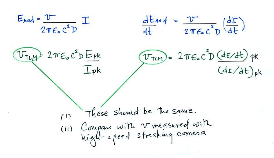
We're going to take a very quick look at another lightning return stroke model, the traveling current source (TCS) model because it predicts that velocities determined using derivative values will be larger than when E and I values are used. The TCS model also has some physically realistic features.
Here just as a reminder and to serve as a comparison is a schematic view of the transmission line model.
For dE/dt, the cable from the flat plate antenna (the left most antenna above) was not connected to an integrator. Rather it was connected to a 50 ohm resistor, the characteristic impedance of the coaxial cable. The voltage that appears across this resistor is proportional to dE/dt as shown below.
Note the dE/dt signal cable is here shown connected to the internal trigger of the storage oscilloscope (the 5 MHz RF signal was also used to trigger the storage oscilloscope). The dE/dt signal then ran through a 45 m length of coaxial cable before being connected to the input of the storage oscilloscope. The 45 m length of cable acted as a delay line (about 150 ns of delay). The hope was that with sufficient "pretrigger" signal you could establish an accurate zero. The figure below shows an oscilloscope display of a signal with and without delay.
 |
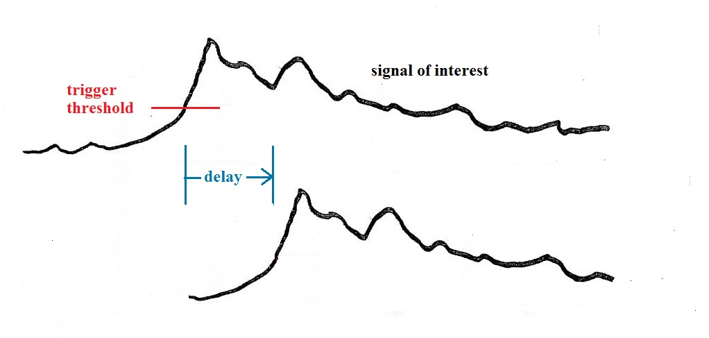 |
The oscilloscope begins to sweep when the signal crosses the trigger threshold. Without delay you would only capture a portion of the rise to peak (left figure). With sufficient delay (right figure) you could capture the entire front edge of the signal.
Some examples of dE/dt signals recorded with a system like the one above are shown below at left. An E signal obtained by integrating the dE/dt waveforms is shown at right. LS and RS indicate leader step and return stroke signals respectively.
The dE/dt signals were recorded on a very fast time base. A storage oscilloscope was oscilloscope signal if a storage scope hadn't been used. The red line shown at the left of each of the dE/dt signals shows the approximate storage oscilloscope trigger level.
As best I can remember the waveform digitizers above had the following characteristics
| Model number |
resolution |
maximum sampling rate |
memory size |
| Biomation 805 |
8 bits |
5 MHz (0.2 μs/sample) |
2048 |
| Biomation 1010 |
10 bits |
10 MHz (0.2 μs/sample) | ? |
| Biomation 8100 |
8 bits |
100 MHz (10 ns/sample) |
? |
| Biomation 1015 |
? |
100 kHz (10 μs/sample) | ? |
The Traveling Current Source lightning return stroke current model
You may remember in the experimental test of the transmission line model that simultaneous measurements of Epeak and Ipeak and also (dE/dt)peak and (dI/dt)peak were made. The measured values were inserted into the transmission line model equations and we solved for the return stroke velocity, vTLM. We should have gotten the same velocity regardless of whether E & I or dE/dt & dI/dt were used. That didn't turn out to be the case. The velocity value obtained using dE/dt and dI/dt was larger than when E and I were used.
We're going to take a very quick look at another lightning return stroke model, the traveling current source (TCS) model because it predicts that velocities determined using derivative values will be larger than when E and I values are used. The TCS model also has some physically realistic features.
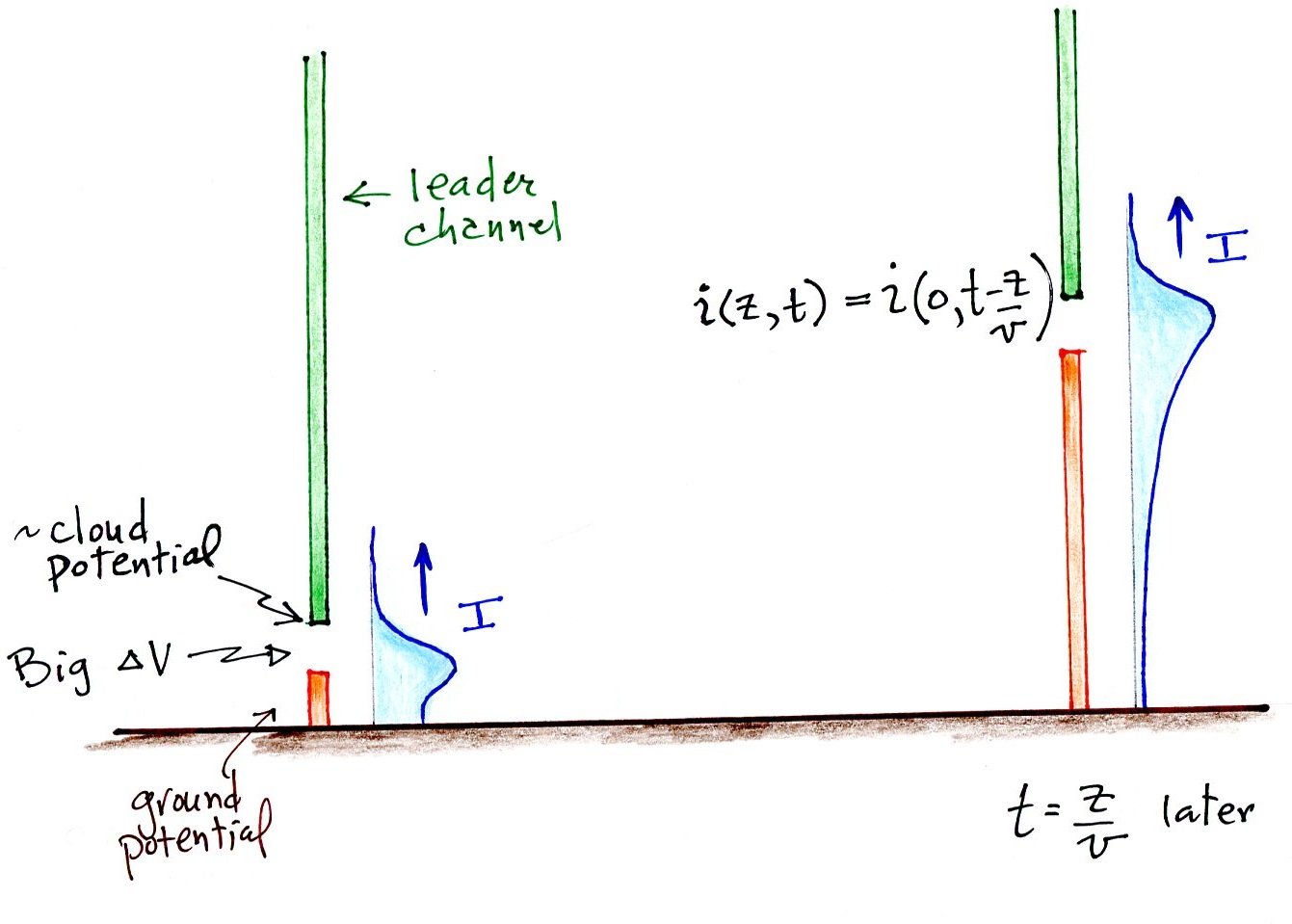
Here just as a reminder and to serve as a comparison is a schematic view of the transmission line model.
The return stroke current begins at the
ground and travels up a vertical channel at constant
speed, v, without changing shape. The current
waveform measured at the ground at the beginning of the
return stroke passes a point z above the ground at t = z /
v.
The new, traveling current source model, is illustrated below.
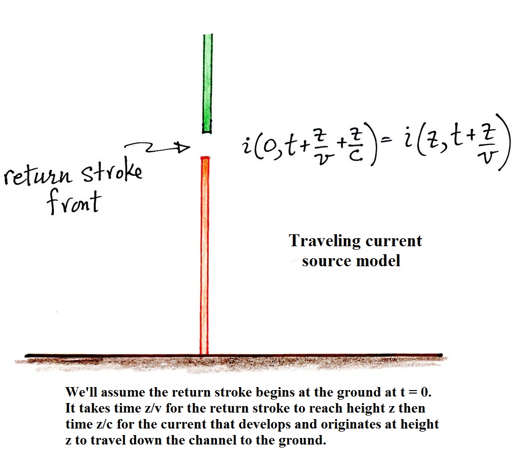
The new, traveling current source model, is illustrated below.
In this model (originally proposed
by Heidler (1985)) current begins not at the ground
but above the ground at the return stroke front as
charge as charge is drained from the leader channel
(charge surrounding the leader channel at about cloud
potential drains into the return stroke channel which
is at ground potential). The current then
travels down the channel to the ground at the speed of
light. The return stroke front is assumed to
propagate upward at constant speed v. The
figures and discussion of the traveling current source
(TCS) model found in this section are taken from
Diendorfer and Uman (1990).
The current that develops at altitude z consists of two components: a "breakdown" current due to relatively rapid draining of charge in the leader head and leader core and a "corona" current due to slower movement of charge surrounding the leader channel.
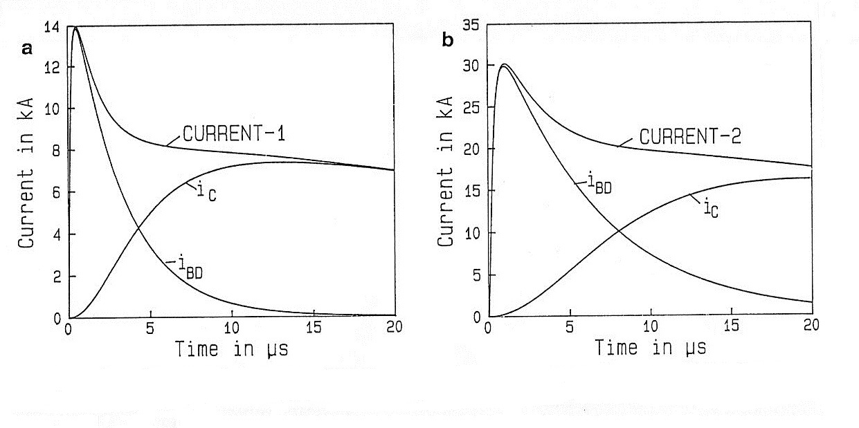
The current that develops at altitude z consists of two components: a "breakdown" current due to relatively rapid draining of charge in the leader head and leader core and a "corona" current due to slower movement of charge surrounding the leader channel.
An illustration of the two
current components in the TCS model (BD is
breakdown and C is corona). The breakdown
component is largely determines the peak E and
peak dE/dt field amplitudes. The Current-1
and Current-2 waveforms in the figure above are
thought to be good approximations of subsequent
and first return stroke current waveforms that
would be observed at the ground.
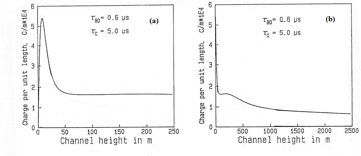
This figure shows the distribution of charge along the leader channel as a function of altitude (the lowest 250 m in (a) and the bottom 2500 m in (b)). Note the buildup of charge at the bottom tip of the leader. This is the charge distribution needed to produce the Channel-1 (subsequent stroke) waveform.
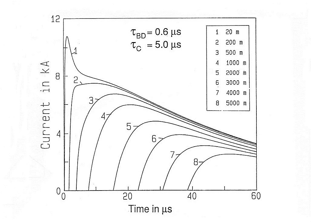
This figure shows the current waveforms that would be observed at different altitudes above the ground (at ground level the Channel-1 waveform peaks at about 14 kA). Changes in signal shape like this are seen in measurements of the optical signals coming from short segments of the return stroke channel at different altitudes above the ground (a topic we might cover later in the semester).
Here is an example of peak E and peak dE/dt values predicted by the TCS model for given peak I and peak dI/dt values together with the velocity values that would be inferred using the transmission line model expressions
Peak I = 14 kA
Peak Erad (at 100 km range) = 2.0 V/m
v = 0.71 x 10⁸ m/s
Peak dI/dt = 75 kA/μsec
Peak dE/dt (at 100 km range) = 27.5 V/m μs
v = 1.83 x 10⁸ m/s
The velocity value derived from peak dI/dt and dE/dt values is larger than the velocity derived from the peak E and I values just as was observed in the Florida experiments. Also we should note that both of the velocity values above (computed using the transmission line model equations) are different from the return stroke front propagation speed of 1.3 x 10⁸ m/s used in the TCS model.
This figure shows the distribution of charge along the leader channel as a function of altitude (the lowest 250 m in (a) and the bottom 2500 m in (b)). Note the buildup of charge at the bottom tip of the leader. This is the charge distribution needed to produce the Channel-1 (subsequent stroke) waveform.
This figure shows the current waveforms that would be observed at different altitudes above the ground (at ground level the Channel-1 waveform peaks at about 14 kA). Changes in signal shape like this are seen in measurements of the optical signals coming from short segments of the return stroke channel at different altitudes above the ground (a topic we might cover later in the semester).
Here is an example of peak E and peak dE/dt values predicted by the TCS model for given peak I and peak dI/dt values together with the velocity values that would be inferred using the transmission line model expressions
Peak I = 14 kA
Peak Erad (at 100 km range) = 2.0 V/m
v = 0.71 x 10⁸ m/s
Peak dI/dt = 75 kA/μsec
Peak dE/dt (at 100 km range) = 27.5 V/m μs
v = 1.83 x 10⁸ m/s
The velocity value derived from peak dI/dt and dE/dt values is larger than the velocity derived from the peak E and I values just as was observed in the Florida experiments. Also we should note that both of the velocity values above (computed using the transmission line model equations) are different from the return stroke front propagation speed of 1.3 x 10⁸ m/s used in the TCS model.
Using triggered
lightning to evaluate performance of the
National Lightning Detection Network
Triggered lightning return
strokes closely resemble the subsequent return
strokes in natural lightning. Most of the
lightning triggered at the International Center
for Lightning Research and Testing (ICLRT) in
north Florida is detected and located by the
National Lightning Detection Network. This
data set can be used to evaluate the performance
of the NLDN (at least the SE portion of the
network). Signal amplitudes measured by the
sensors in the NLDN are also used to make
estimates of lightning return stroke peak
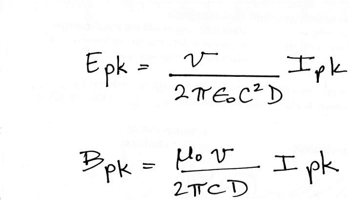
currents. Those estimates make use of the
simple transmission line model expression that
relates peak current I and the peak amplitude of
the electric and magnetic radiation fields (both E
and B fields are measured by the sensors in the
NLDN). We will look at these peak current
estimates in a little more detail here.
Detection efficiency and location accuracy will be
examined in a later class (the Wed., Apr. 8 class it
turns out).
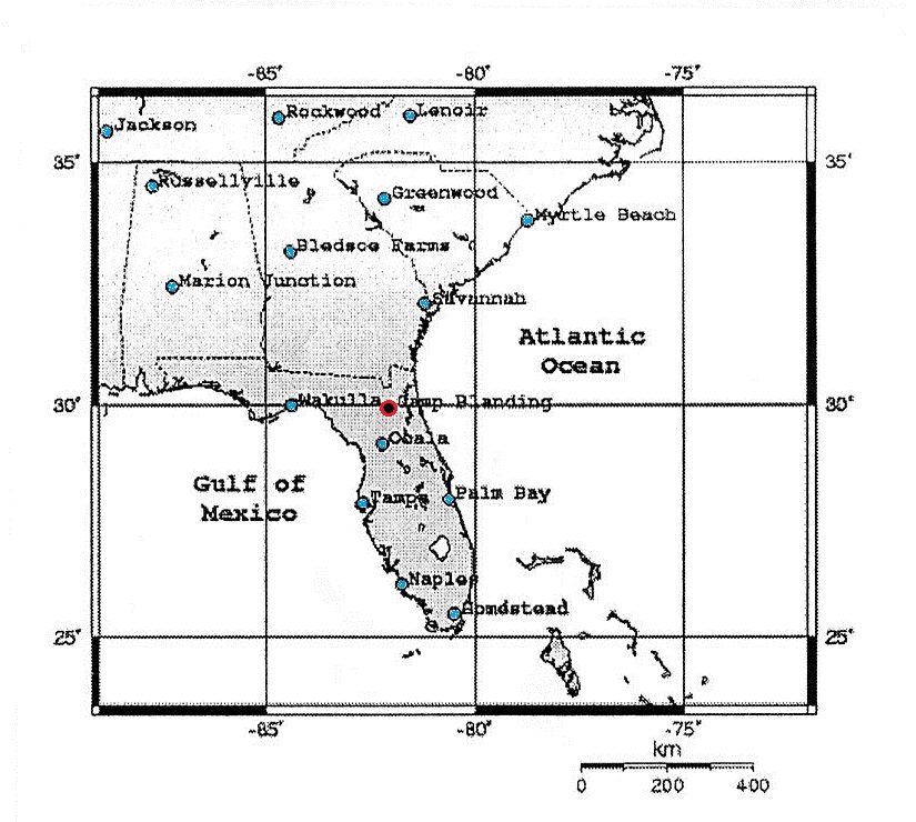
A map showing the locations of
stations in the National Lightning Detection
Network near the International Center for
Lightning Research and Testing at Camp Blanding,
Florida.
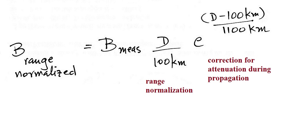
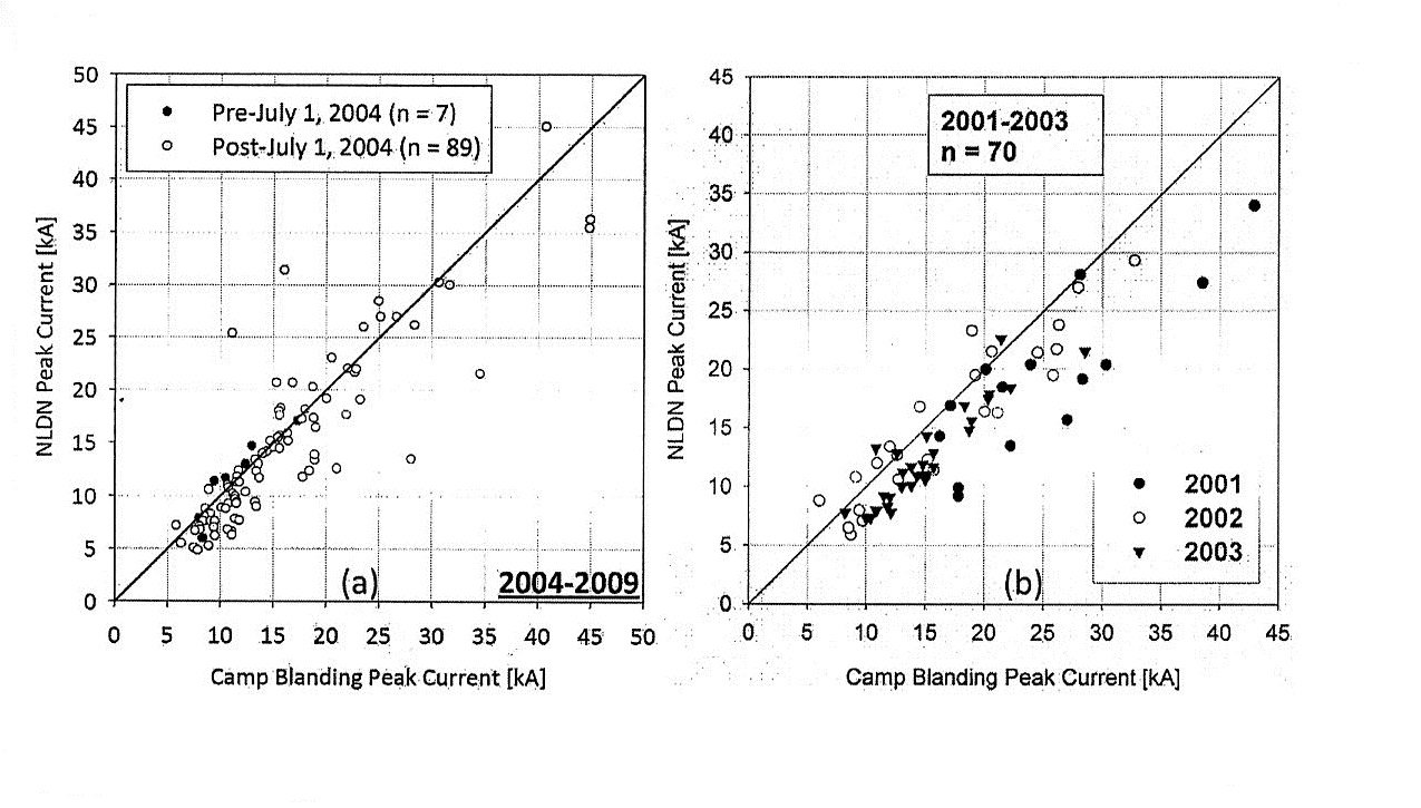
Lightning triggered at Camp Blanding was detected and located by the NLDN network. These data could be used to evaluate the detection efficiency and location accuracy of this portion of the NLDN. Magnetic field signals detected at the NLDN sensors are used to estimate lightning return stroke peak currents. These estimates could be compared with direct measurements of current made at the lightning triggering site.
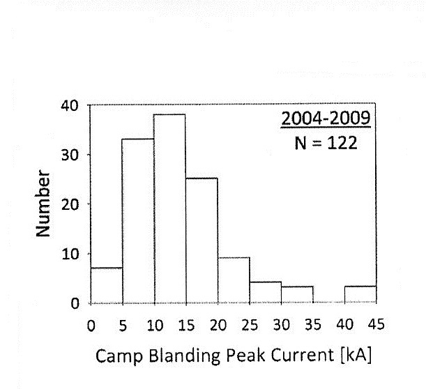
Lightning triggered at Camp Blanding was detected and located by the NLDN network. These data could be used to evaluate the detection efficiency and location accuracy of this portion of the NLDN. Magnetic field signals detected at the NLDN sensors are used to estimate lightning return stroke peak currents. These estimates could be compared with direct measurements of current made at the lightning triggering site.