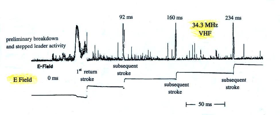
Most lightning discharge processes are strong emitters of VHF radiation. This is evident on the figure above which shows VHF emissions and a slow E field record of a multi-stroke cloud-to-ground discharge. When we examine the VHF radiation on a faster time scale however we see that the VHF signals can broadly divided into two groups. First sequences of isolated pulses of roughly 1 μs duration and bursts of "quasi-continuous" emission that last for 10s of microseconds or more. Examples of both types of signals are shown in the figure below adapted from Proctor (1988).
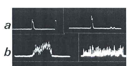
On Row (a) are examples of the isolated pulses. Signals of this type are produced by discharge processes that propagate into unionized air and are best located by TOA systems. Examples of quasi-continuous radiation are shown Row (b) (Proctor refers to these types of signals as "Q-noise"). The two bursts in the figure lasted 30 μs and 45 μs This type of radiation seems to be produced by return strokes and recoil streamers, i.e. a discharge process that travels along an existing channel. Interferometry is best able to locate the sources of this radiation.
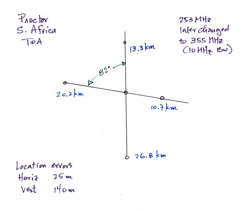
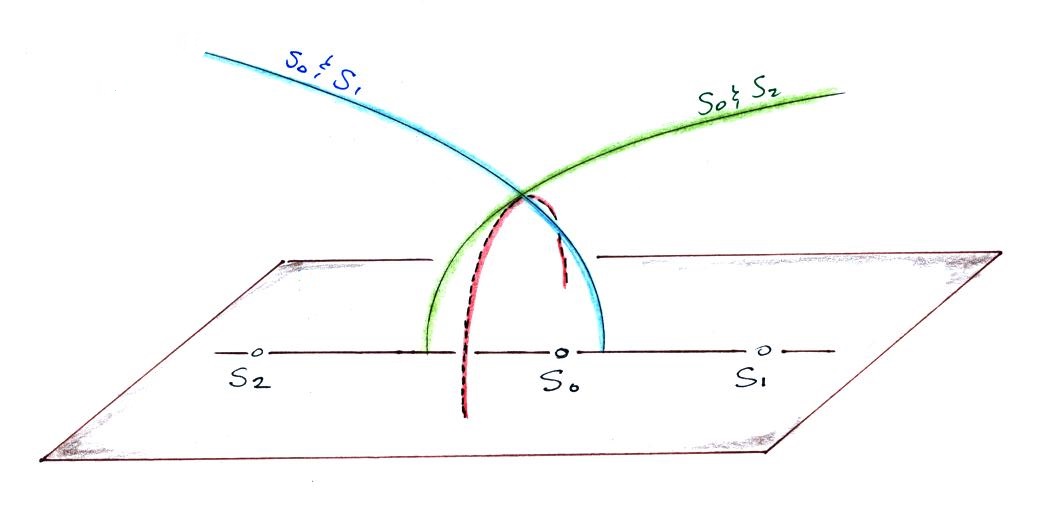
Probably the first 3-D TOA location system used for lightning research was D.E. Proctor's South African network. It is shown below and is described in more detail in Proctor (1971). This is a long baseline system where the distance between receivers (a few 10s of km in this case) is much greater than the wavelength of the VHF radiation.
In Proctor's sytem, four 253 MHz receivers (later changed to 355 MHz) were positioned at the ends of two nearly perpendicular baselines. A fifth receiver was positioned in the center at the intersection of the two baselines. Signals received at the four outer stations were transmitted to the center station by microwave link. Because the time of propagation from the outer stations to the center station could be accurately determined, the time of the arrival of signals at the outer stations could be determined very precisely.
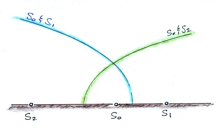
Though because we are now working in 3 dimensions, each of the hyperbolae should be rotated around the baseline connecting the stations.
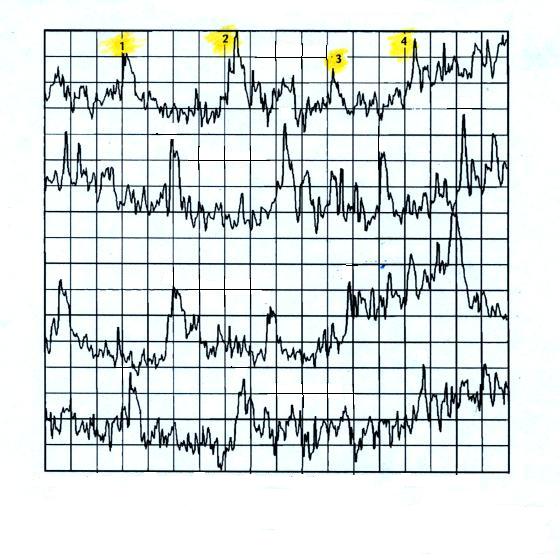
An example of RF data from the 5 receivers is shown below (from Proctor, 1983). The records are approximately 60 microseconds long.
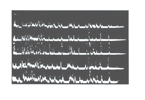
Waveform digitizers were not fast enough at that time to be able to record data like this. So the RF signals from the 5 stations were initially recorded on a cathode ray tube and photographed (a specially designed "laser optical recorder" was later used to record the data directly onto film). In the example above, the data recorded on film have been digitized and displayed on a computer for analysis.
In order to locate an emission source in space you must first identify the correlated RF impulses on the 5 records. The records can be complex with signals from multiple sources arriving at the different receivers in different order. This analysis was originally done by hand and could be quite tedious (the following quotes are from Proctor 1981, I added the underlines)
"Even those who enjoy reading reading records that can be deciphered easily found that reading the more complicated variety was a mild from of torture, and that it took about one man-month's effort to locate 100 sources correctly."
On average it was possible to locate the source of one pulse in every 70 microseconds of record.
We'll look at just one example of many interesting results obtained with the South African VHF TOA network. Proctor (1991) determined where lightning discharges began by finding the centroid of the first 6 to 10 VHF pulse locations emitted in a flash. The left figure below shows origin heights (above ground level) for 773 cloud-to-ground and intracloud flashes in 13 thunderstorms. Origin heights for 214 cloud-to-ground flashes are shown in the figure at right. The network was 1.43 km above sea level.
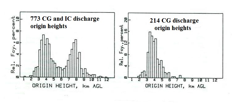
For the lower altitude peak in the left figure, median heights for individual storms ranged from 4.4 km to 5.7 km above mean sea level (amsl) which corresponded to temperatures ranging from +1o C to -8.5o C. Median heights for the 2nd higher altitude peak ranged from 7.5 km to 9.7 km amsl where temperatures ranged from -21.1o C to -33o C.
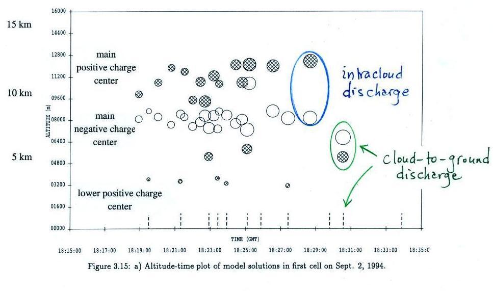
We can refer back to a figure in our Feb. 20 lecture (reproduced below) showing the locations of charge centers involved in cloud-to-ground and intracloud discharges (the charge center locations where derived from E field change measurements made at multiple sites using the field mill network at the Kennedy Space Center).
Next we'll briefly discuss another long baseline VHF TOA network, the Lightning Detection and Ranging (LDAR) system, that has been operating at the NASA Kennedy Space Center since the mid 1970s. The network has undergone several changes and upgrades since it was first installed. The figure below shows the layout of the system that was being used in the 1990s. It consisted of a central station and 6 surrounding stations positioned on roughly a 20 km diameter circle.
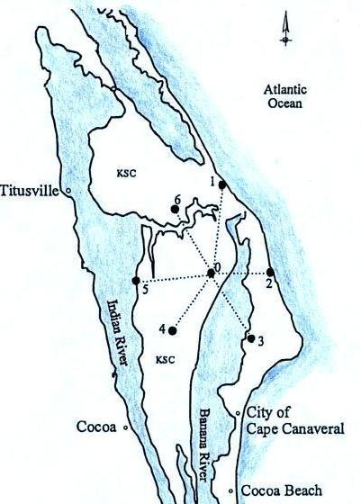
The VHF receivers operate at 66 MHz (6 MHz bandwidth) and data from the remote stations are telemetered back to the center station by microwave link where they are digitized. A signal crossing threshold at the center receiver triggers a roughly 100 μs; long recording at each of the 7 stations. Correlated pulses on the separate records and differences in the times of arrival are found using pattern recognition and cross correlation techniques. TOA data from the center station and 3 of the outer stations (stations 0, 1,3, and 5 for example) are used to determine an RF source location. A second location is determined using the center data and the other 3 remote locations (stations 0, 2, 4 and 6). If the two locations agree the location is accepted.
Here is an example of VHF source locations provided by the LDAR network (from Rustan et al., 1980).
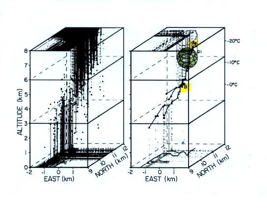
VHF noise began 4.9 ms before the 1st return stroke. The first 2.2 ms was considered preliminary breakdown activity and was followed by the stepped leader which lasted 2.7 ms. The left figure above shows 422 noise sources located during the first 4.7 ms of the flash. The right figure plots locations at 94 μs intervals during the preliminary breakdown (between Pts. A & B which are highlighted in yellow) and the stepped leader (below Pt. B). Q1 is the charge transported to ground during the first return stroke in this flash (determined from field change records using the methods discussed in the Feb. 20 lecture mentioned above). Four additional plots like this tracing out activity during the remainder of the discharge can be found in Rustan et. al (1980).
We'll next consider the most recent and most advanced VHF TOA system, the Lightning Mapping Array (LMA) developed by researchers at the New Mexico Institute of Mining and Technology (New Mexico Tech). The system detects 60-66 MHz radiation (television channel 3).
The system was originally used in Oklahoma in June 1998 (a map of sensor locations can be found here and results from the Oklahoma field experiment can be found here or here) and then in New Mexico in August and September. The New Mexico network, as described by Rison et. al (1999), consisted of 10 stations that were deployed over an area about 60 km in diameter near Langmuir Laboratory. Quoting from the Rison et. al article: "The time and magnitude of the peak radiation is recorded during every 100 μs time interval that the RF power exceeds a noise threshold." The time of the peak signal is recorded with 50 ns resolution. TOA information from events strong enough to be detected at six or more stations are located in space and time. This TOA information is determined at each of the remote stations and the information is sent back to a central location (rather than transmitting the raw VHF data back to a base station).
It is a little difficult to keep up with the rapid development and results coming from the LMA. As best I can tell (2012 source, newer source) permanent and operational LMAs can be found in or at the NASA Marshall Space Flight Center in Alabama (see also this link), the National Weather Service in Washington DC, Oklahoma, Texas A&M University near Houston, West Texas (Texas Tech University), Displays of real time data are available online at many of these sites. Here's a link to a useful site with a variety of lightning related resources.
Some photographs of an early version of the system being demonstrated in the Washington DC area are shown below (source of these images)
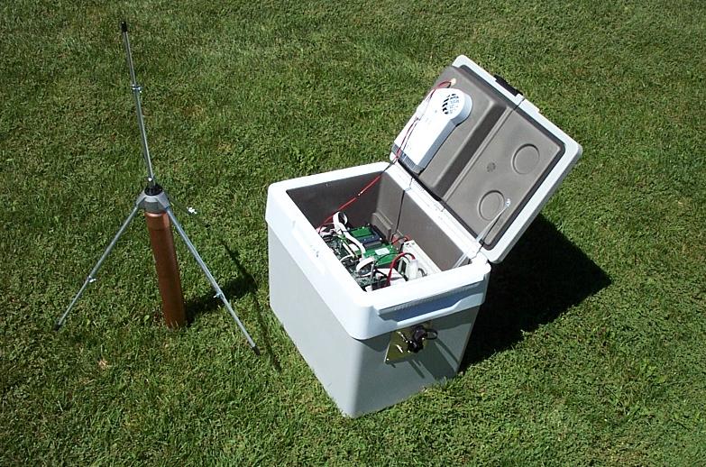
VHF antenna and open electronics enclosure showing the electronics (a more detailed photograph of the electronics can be found here)
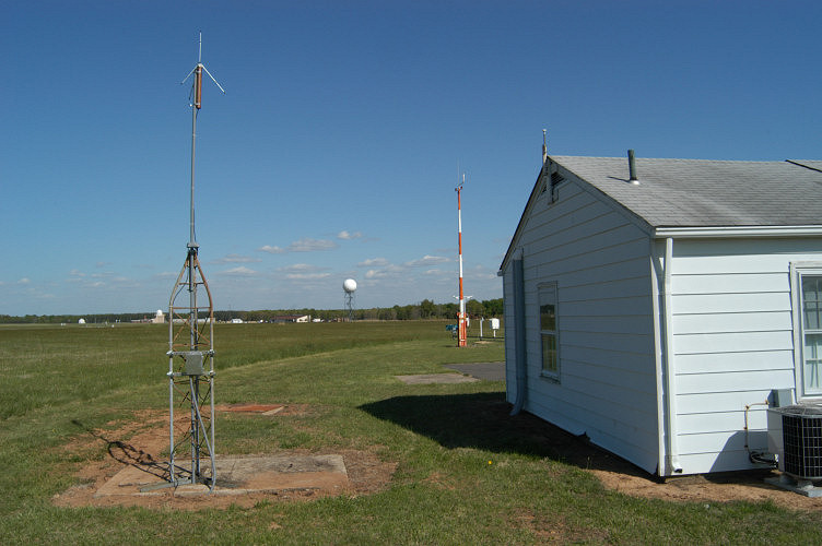
VHF antenna installation at the Sterling VA location.
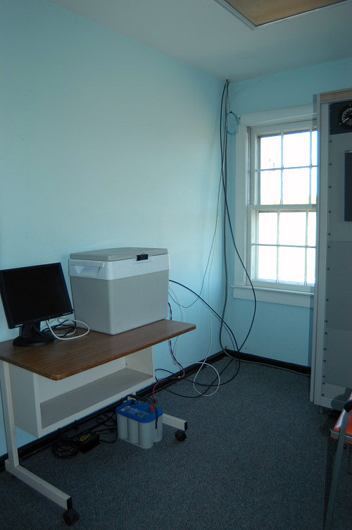
Electronics enclosure.
Here are some animations of lightning activity located with the Oklahoma LMA. The links and explanation of the format of the data display below have been copied from http://lightning.nmt.edu/nmt_lms/ok98.html.
|
 The top t vs. z plot shows all the points located in the given time interval. The time is given in seconds, and the altitude z of the radiation source is given in kilometers. The number of points can be limited if desired. For example, two distinct discharges at different locations could occur at the same time, so the operator may choose to look at only one of the dishcarges in detail. Or the operator may narrow in on a particular event in time which he does not want obsured by other data points. The lower four plots show data points from the top plot which have been selected for such reasons. The lower t vs. z plot shows the time development of the altitude of the selected points. The x vs. y plot shows a plan view of the lightning discharge, where x is the distance east or west of the center of the array, and y is the distance north or south of the center. All distances are given in kilometers. The small squares in the x vs. y plot show the locations of the LMA stations. The x vs. z and y vs. z plots show the projections of the points on the xz and yz planes.
Discharge showing distinct
charge layers at different
elevations. Note the development
of the dendritic structure of
the discharge.
11 June 1998 06:33:20 UTC (645 KB Animated GIF) Cloud-to-ground
discharge followed by intercloud
discharge. Note the well-defined
leaders in the CG. The triangles
are locations and times of CG
strokes as determined by the
National Lightning Detection
Network. Note that, in the CG,
positive streamers propagate in
the negative charge region,
radially away from the area of
initial breakdown. The
subsequent IC develops over the
top of of the CG.
11 June 1998 06:19:39 UTC (1.5 MB Animated GIF)
Discharge
near the end of a storm which
appears to be inverted. There
are two distinct charge layers,
but streamers appear to
originate in the upper layer and
propogate to the lower layer.
This is inverted from most
intercloud discharges in which
negative streamers originate in
the lower negative charge layer
and propogate into the upper
positive charge layer. Also note
how the lower charge region
decreases in altitude to the
east.
20 June 1998 03:43:45 UTC (1.8 MB Animated GIF) |
Finally, be sure to look at this very cool animation of a lightning flash over New Mexico near Langmuir Lab that is on YouTube.
The section discussing locating lightning VHF sources using interferometry has been moved to the Friday April 10 notes.
Proctor, D.E., "A Hyperbolic System for Obtaining VHF Radio Pictures of Lightning," J. Geophys. Res., 76, 1478-1489, 1971.
Proctor, D.E., "VHF Radio Pictures of Cloud Flashes," J. Geophys. Res., 86, 4041-4071, 1981.
Proctor, D.E., "Lightning and Precipitation in a Small Multicellular Thunderstorm," J. Geophys. Res., 5421-5440, 1983.
Proctor, D.E., R. Uytenbogaardt, B.M. Meredith, "VHF Radio Pictures of Lightning Flashes to Ground," J. Geophys. Res., 93, 12683-12727, 1988.
Proctor, D.E., "Regions Where Lightning Flashes Begin," J. Geophys. Res., 96, 5099-5112, 1991.
Rison, W. R.J. Thomas, P.R. Krehbiel, T. Hamlin, and J. Harlin, "A GPS-based Three Dimensional Lightning Mapping System: Initial Observations in Central New Mexico," Geophys. Res. Lett., 26, 3573-3576, 1999. (you should find a link to a pdf version of the document)
Rustan, P.L., M.A. Uman, D.G. Childers, and W.H. Beasley, "Lightning Source Locations From VHF Radiation Data for a Flash at Kennedy Space Center," J. Geophys. Res., 85, 4893-4903, 1980.
Uman, M.A., W.H. Beasley, J.A. Tiller, Y-T. Lin, E.P. Krider, C.D. Weidman, P.R. Krehbiel, M. Brook, A.A. Few, J.L. Bohannon, C.L. Lennon, H.A. Poehler, W. Jafferis, J.R. Gulick, J.R. Nicholson, "An Unusual Lightning Flash at Kennedy Space Center," Science, 201, 9-16, 1978.