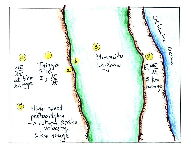
Point 1 is the location of the
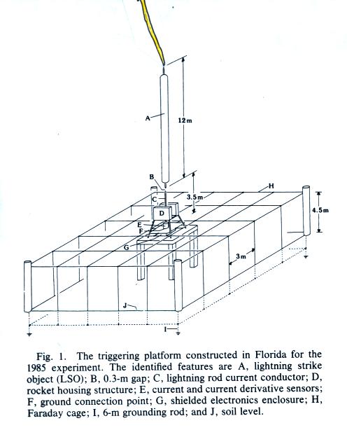
triggering site. A rather complicated launch platform
was in place during the 1985 experiments which may have
affected the measurements and interpretation of the results
(Point 1a in the figure above and the left figure below which
is from "Current
and Electric Field Derivatives in Triggered Lightning Return
Strokes," C. Leteinturier, C. Weidman, and J. Hamelin, J.
Geophys. Res., 95, 811-828, 1990.).
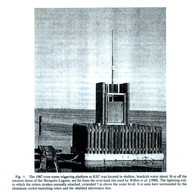
About as "clean" a launch platform as could be imagined was
used in 1987 (Point 1b in the figure above and the right
photograph below from "Submicrosecond
Intercomparison
of
Radiation
Fields
and
Currents
in
Triggered
Lightning
Return
Strokes
Based
on
the
Transmission-Line
Model,"
J.C.
Willett,
J.C.
Bailey,
V.P.
Idone,
A.
Eybert-Berard,
and
L.
Barret,
J.
Geophys.
Res.,
94,
13275-13286, 1989.).
E and dE/dt fields were recorded at Point 2, 5 km from the triggering site. At this range and at the time of peak E and peak dE/dt it is safe to assume the measured E fields were purely radiation fields. The Mosquito Lagoon is filled with brackish water, a mixture of fresh water and salty ocean water. So propagation between the triggering site and the E field antennas was over a relatively high conductivity surface and high frequency signal content was preserved. The effects of propagation will be discussed in a little more detail later in the lecture.
E field derivative signals were also recorded at Point 4, 50 meters from the trigger point. At this close range the dE/dt signals probably did contain induction and electrostatic field components and using them to infer peak dI/dt values using the transmission line model is probably not valid.
Finally return stroke velocities were measured using high-speed streaking cameras at Point 5, located 2 km from the triggering point.
 |
 |
E and dE/dt fields were recorded at Point 2, 5 km from the triggering site. At this range and at the time of peak E and peak dE/dt it is safe to assume the measured E fields were purely radiation fields. The Mosquito Lagoon is filled with brackish water, a mixture of fresh water and salty ocean water. So propagation between the triggering site and the E field antennas was over a relatively high conductivity surface and high frequency signal content was preserved. The effects of propagation will be discussed in a little more detail later in the lecture.
E field derivative signals were also recorded at Point 4, 50 meters from the trigger point. At this close range the dE/dt signals probably did contain induction and electrostatic field components and using them to infer peak dI/dt values using the transmission line model is probably not valid.
Finally return stroke velocities were measured using high-speed streaking cameras at Point 5, located 2 km from the triggering point.
Here's the basic idea behind
the experiment. The transmission line model predicts
that the current waveform (I) and the electric radiation
field waveform (E) (also dI/dt and dE/dt) will have
identical shapes similar to what is drawn below.
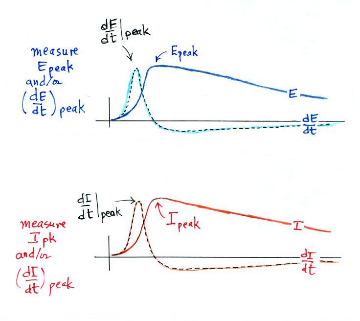
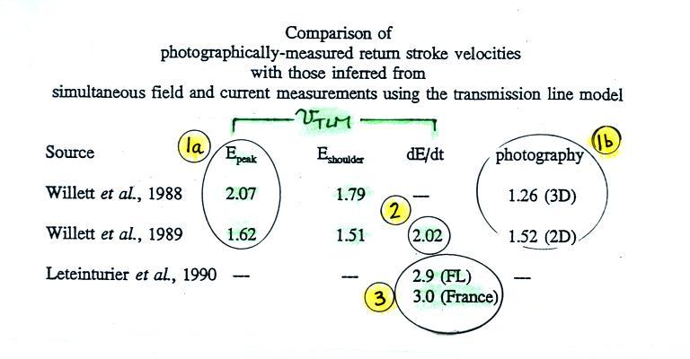
We measure Epeak and Ipeak and also (dE/dt)peak and (dI/dt)peak. We then insert these measurements into the transmission line model equations. D, the distance between the strike point and the locations where the field measurements were made, was known. We solve for the return stroke velocity, vTLM.
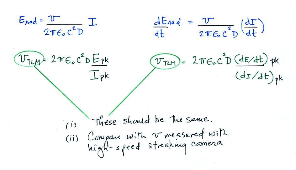
It shouldn't matter whether you use E and I data or dE/dt
and dI/dt measurements, the value of vTLM
should be the same.
The transmission line model derived
velocity, vTLM
, was then compared with the velocity measured with the
high-speed streaking camera. The next figure shows
how things turned out. (the velocity values in the
table should all be multiplied by 108 m/s)We measure Epeak and Ipeak and also (dE/dt)peak and (dI/dt)peak. We then insert these measurements into the transmission line model equations. D, the distance between the strike point and the locations where the field measurements were made, was known. We solve for the return stroke velocity, vTLM.
Let's first look at Points
1a and 1b. Point 1a shows vTLM
determined
using the E and I measurements and the transmission line
model expression. Point 1b shows the measurements of
return stroke velocity made with the streak camera.
The value of vTLM
obtained for the 1985 experiment 2.07 does not
agree very well with the measured value 1.26. This
may be due to the complicated launch platform.
Agreement was a little better for the 1987 experiment
(1.62 vs 1.52). A student in class wondered whether
the differences between v and vTLM
might have been due to the fact that 3-dimensional
velocities were measured in 1985 and 2-D velocities were
measured in 1987. My feeling is that this wouldn't
explain the differences. Because we are looking at
velocity in the bottom of a triggered lightning channel,
which is probably pretty straight and vertical, I don't
think there will be much difference between the 2-D and
3-D velocities.
At Point 2 we can see that vTLM using dE/dt and dI/dt is higher than the vTLM determined using E and I. This discrepancy has not been explained. The velocity values at Point 3 are appreciably higher than any of the other values. This estimate of vTLM was determined using dE/dt measured at 50 m distance from the triggering point. As we mentioned earlier, these fields probably contain induction and electrostatic field contributions and the transmission line model expression should probably not be used in this case.
We haven't explained the Eshoulder column in the table yet. A careful comparison of I and Erad signals on a fast time scale (which the transmission line model predicts should be identical) shows some subtle differences between the two waveform shapes. Rather than just a single peak, the Erad signal often has a second somewhat smaller peak or shoulder as sketched below.
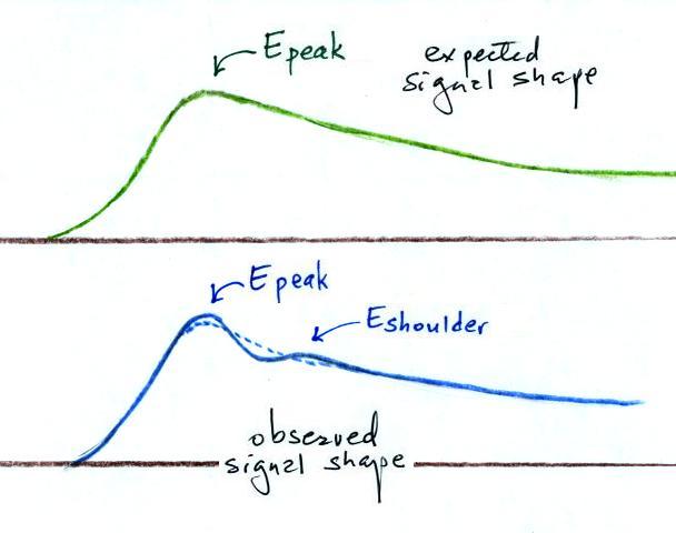
Much better agreement between vTLM and measured velocities was obtained when the Eshoulder amplitude was used with Ipeak in the transmission line expression when computing vTLM.
Now we'll look at one possible explanation of the Eshoulder feature (we mainly follow the discussion in the Leteinturier (1990) paper mentioned earlier)
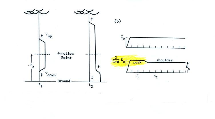
We ordinarily think of the return stroke as being a single upward propagating current that begins at the ground. This view is shown in the figure below. Let's say a peak current of Io at the ground produces a field with a peak value Eo at some distance from the strike point.
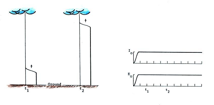
It may be that the return stroke doesn't begin at the ground but a few 10s of meters above the ground at the junction point between the upward connecting discharge and the stepped leader. In this case there might not be just a single upward propagating current, rather currents might travel up and down from the junction point.
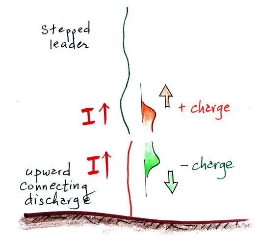
When the downward wave reaches the ground it may be partially reflected. This kind of a situation, together with a few assumptions, can produce an E field signal that resembles the peak and shoulder features seen in the triggered lightning data.
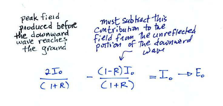
We need to look at this in a little more detail to be able to explain the field values in the right figure above. We'll first assume that the current rises to peak value before the downward wave reaches the ground. The waves might travel at 1/3 the speed of light, 1 x 10⁸ m/s. If the current peaks in 0.1 microseconds, the junction point would need to be at least 10 m above the ground. If it takes 1 microsecond for the current to reach peak the junction point would need to be 100 m high (that seems a bit much).
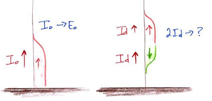
A single upward propagating current with amplitude Io will produce a radiation field with amplitude Eo. What field will two current waves each with amplitude Id produce? We need to find some relation between Id and Io. To do that we need to look at what happens when the downward traveling wave reaches the ground. This is sketched in the figure below.
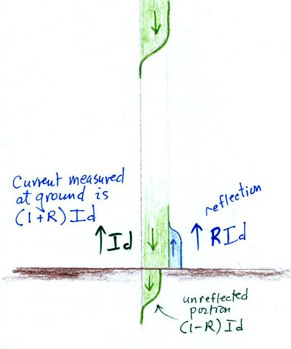
The top part of the figure shows the downward current wave moving toward the ground. At the bottom of the figure we show what happens when the wave reaches the ground. A portion of the downward wave is reflected (shown in blue). We will assume that the reflected current wave, which has amplitude R Id, and the original wave, with amplitude Id, add. In a measurement of current at the ground we wouldn't be able to separate the two contributions to the current (downward and reflected waves)
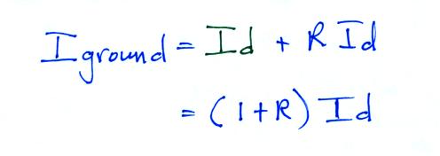
We will force Iground to be equal to Io
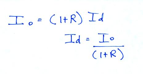
so that from the point of view of the current being measured at the ground, the two versions of return stroke initiation (a single upward propagating current wave that starts at the ground versus upward and downward pointing current waves that start at a junction point above the ground) are indistinguishable. The same current waveform would be measured at the ground in both cases.
Now that we can relate Id and Io we can go back to our earlier figure
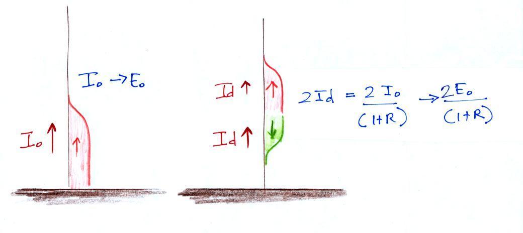
One current wave with amplitude Io produces a field Eo. Two current waves, each with amplitude Id, produce a field with a peak value of 2Eo/(1+R). So we've explained part of the figure below (the amplitude of the E field peak highlighted in yellow).
At Point 2 we can see that vTLM using dE/dt and dI/dt is higher than the vTLM determined using E and I. This discrepancy has not been explained. The velocity values at Point 3 are appreciably higher than any of the other values. This estimate of vTLM was determined using dE/dt measured at 50 m distance from the triggering point. As we mentioned earlier, these fields probably contain induction and electrostatic field contributions and the transmission line model expression should probably not be used in this case.
We haven't explained the Eshoulder column in the table yet. A careful comparison of I and Erad signals on a fast time scale (which the transmission line model predicts should be identical) shows some subtle differences between the two waveform shapes. Rather than just a single peak, the Erad signal often has a second somewhat smaller peak or shoulder as sketched below.
Much better agreement between vTLM and measured velocities was obtained when the Eshoulder amplitude was used with Ipeak in the transmission line expression when computing vTLM.
Now we'll look at one possible explanation of the Eshoulder feature (we mainly follow the discussion in the Leteinturier (1990) paper mentioned earlier)
We ordinarily think of the return stroke as being a single upward propagating current that begins at the ground. This view is shown in the figure below. Let's say a peak current of Io at the ground produces a field with a peak value Eo at some distance from the strike point.
It may be that the return stroke doesn't begin at the ground but a few 10s of meters above the ground at the junction point between the upward connecting discharge and the stepped leader. In this case there might not be just a single upward propagating current, rather currents might travel up and down from the junction point.
When the downward wave reaches the ground it may be partially reflected. This kind of a situation, together with a few assumptions, can produce an E field signal that resembles the peak and shoulder features seen in the triggered lightning data.
We need to look at this in a little more detail to be able to explain the field values in the right figure above. We'll first assume that the current rises to peak value before the downward wave reaches the ground. The waves might travel at 1/3 the speed of light, 1 x 10⁸ m/s. If the current peaks in 0.1 microseconds, the junction point would need to be at least 10 m above the ground. If it takes 1 microsecond for the current to reach peak the junction point would need to be 100 m high (that seems a bit much).
A single upward propagating current with amplitude Io will produce a radiation field with amplitude Eo. What field will two current waves each with amplitude Id produce? We need to find some relation between Id and Io. To do that we need to look at what happens when the downward traveling wave reaches the ground. This is sketched in the figure below.
The top part of the figure shows the downward current wave moving toward the ground. At the bottom of the figure we show what happens when the wave reaches the ground. A portion of the downward wave is reflected (shown in blue). We will assume that the reflected current wave, which has amplitude R Id, and the original wave, with amplitude Id, add. In a measurement of current at the ground we wouldn't be able to separate the two contributions to the current (downward and reflected waves)
We will force Iground to be equal to Io
so that from the point of view of the current being measured at the ground, the two versions of return stroke initiation (a single upward propagating current wave that starts at the ground versus upward and downward pointing current waves that start at a junction point above the ground) are indistinguishable. The same current waveform would be measured at the ground in both cases.
Now that we can relate Id and Io we can go back to our earlier figure
One current wave with amplitude Io produces a field Eo. Two current waves, each with amplitude Id, produce a field with a peak value of 2Eo/(1+R). So we've explained part of the figure below (the amplitude of the E field peak highlighted in yellow).
Now
we need to explain why the field
decreases and forms a shoulder and why
the shoulder amplitude is Eo. To
do that we need to consider the
unreflected portion of the current
wave.
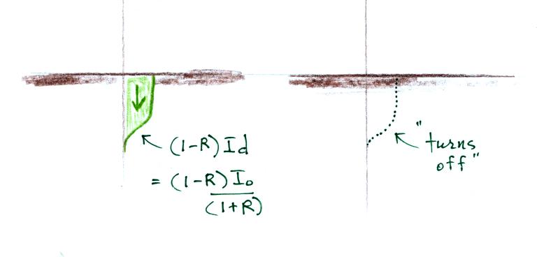
The
unreflected current doesn't just
travel down into the ground as shown
in the figure. It probably
spreads out horizontally. In
any event, as a field emitter, it
"turns off" and stops radiating (it
is traveling into a
conductor). So we need to
subtract its contribution to the
total E field.
So the drop from peak field
to a shoulder field occurs when the
downward current wave reaches the
ground and a portion of the downward
current stops radiating.
Let's go back to our summary of the results of the experimental test of the transmission line model.
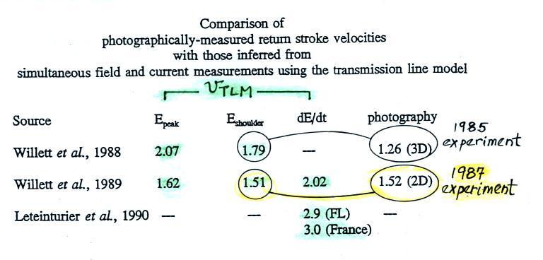
Much better agreement between transmission line model derived velocities and measured velocities was obtained when the Eshoulder amplitude was used instead of Epeak in the transmission line model equation together with Ipeak This is particularly true for the 1987 experiment with its simpler launch platform. Keep the 1.51 x 10⁸ m/s and the 2.02 x 10⁸ m/s velocity values in mind, we'll being referring to them again shortly in the final section in today's notes.
We should note that we still haven't explained why a different vTLM was obtained when using dE/dt and dI/dt data. The transmission line model can't account for this difference. There is another lightning return stroke current model, the so called Traveling Current Source model that does produce a difference like this. We may discuss that model briefly in a future lecture.
We'll end this lecture with a look at some experimental measurements of distant electric radiation fields and estimates of peak I and peak dI/dt values that were derived from them. The measurements are described in the publication cited below.
"Submicrosecond fields radiated during the onset of first return strokes in cloud-to-ground lightning," E.P. Krider, C. Leteinturier, and J.C. Willett, J. Geophys. Res., 101, 1589-1597, 1996.
Here are some important points regarding this experiment.
1. Electric fields from lightning first return strokes 25 to 45 km away were measured. Only the radiation field component is present at these ranges. Propagation between the strike point and the recording station was entirely over salt water so that high frequency signal content was largely preserved. The recording station was actually one of the stations used in the triggered lightning experiment described above (Point 2 on the map at the start of today's lecture)
2. The recording instrumentation was triggered on an RF signal rather than on E or dE/dt to prevent trigger bias.
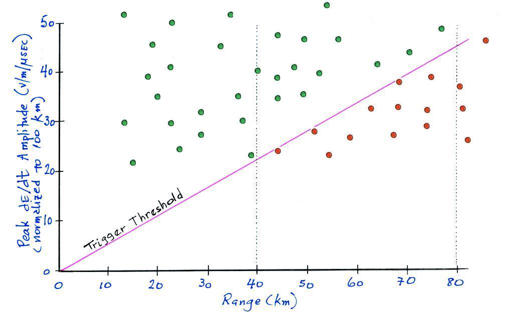
The plot above shows range normalized dE/dt data versus range. A trigger threshold on an oscilloscope or waveform recorder, a fixed voltage, will correspond to larger and larger dE/dt values with increasing range. Between about 40 and 80 km the distribution of measured dE/dt signals will be biased toward larger signal amplitudes. Only the green points on the plot above which are above the trigger threshold would be recorded, beyond about 80 km very few of the dE/dt signals would be large enough to trigger the recording instrumentation. (This is a realistic but fictitious data set being used for illustration, both in the figure above and the histogram below).
The histograms below show the effect of trigger level bias on the distribution of range normalized dE/dt measurements. The first histogram plots the range normalized dE/dt measurements between 40 and 80 km which triggered the recording system. The mean value was 44 V/(m μsec).
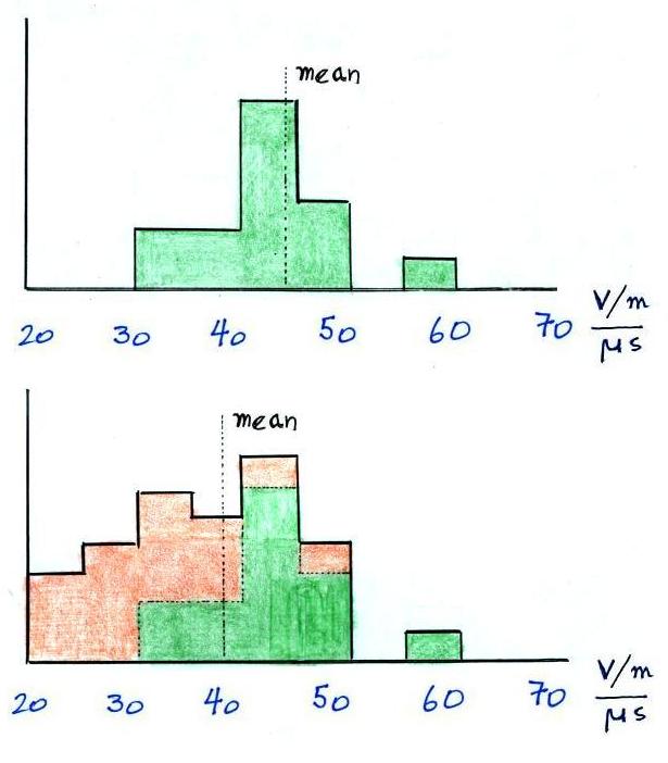
The bottom histogram is the true distribution. I.e. it includes the data that triggered the recording system and those that did not. Including the latter group of data lowers the mean to 38 V/(m μsec).
The table below illustrates how measured dE/dt values can be range normalized.
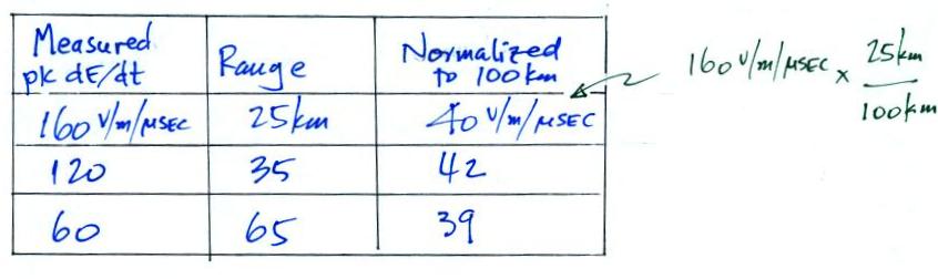
Three typical peak
dE/dt values from return strokes
at ranges of 25, 35, and 65 km
are shown in the left most
column. We assume the
signals vary as 1/range.
Data range normalized to 100 km
are shown in the right
column.
3. Even though E field propagation was over salt water some high frequency attenuation was still present. An attempt was made to correct for this.
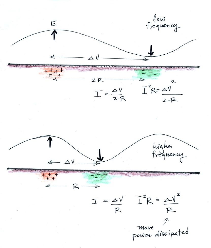
Here's one simple explanation of why the higher frequency signals are preferentially attenuated as they pass over a surface with finite conductivity.
Two signals with the same amplitude, but a factor of 2 difference in wavelength and frequency, are shown. The signals will cause charge to be induced on the surface. If we assume a voltage difference Δ V between locations of the + and - charge, currents will begin to flow in the ground. The current created by the signal with lower frequency will be a little smaller than the current created by the higher frequency signal. More power will be dissipated by the current created by the higher frequency signal than the lower frequency signal. This will reduce the amplitude of the higher frequency signal more than the lower frequency signal.
I'm not sure this approach is valid. Here's an alternate explanation.
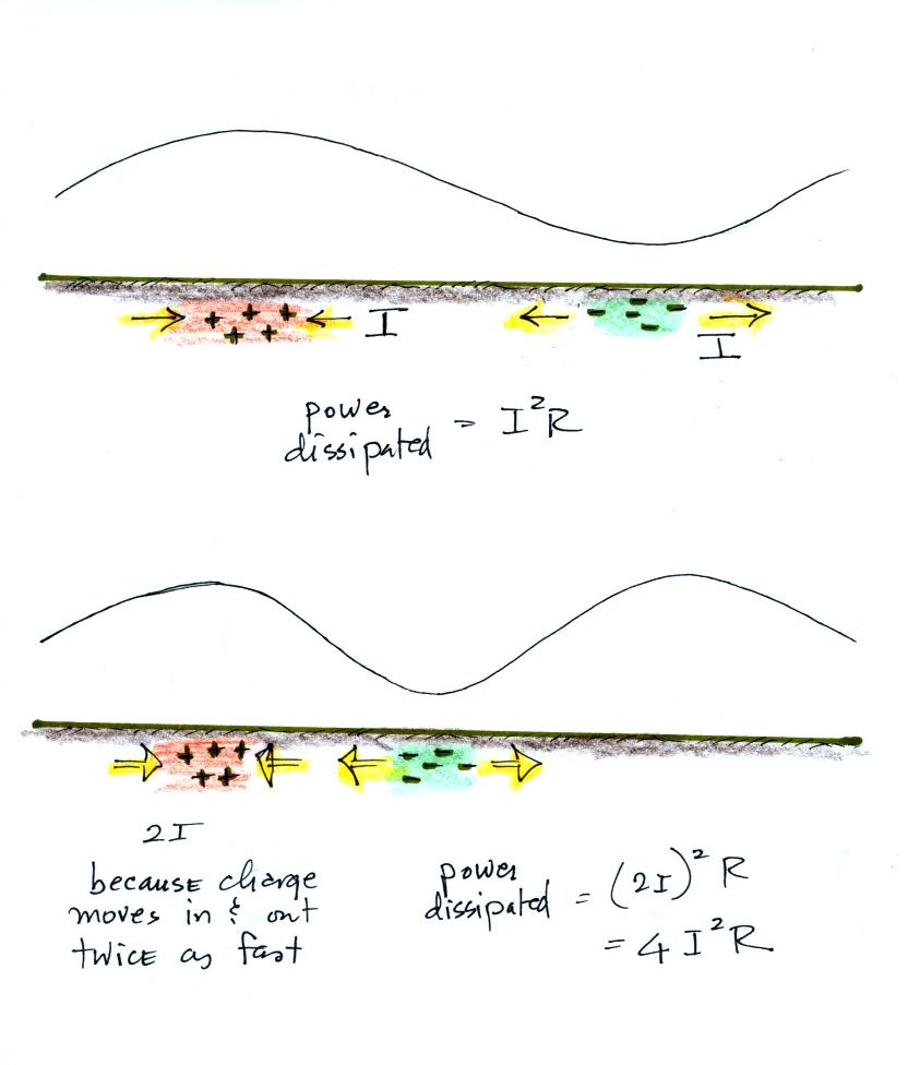
In this case we first
recognize that currents will
flow in the ground as signals
pass over the ground. It
seems reasonable that the higher
frequency signal will cause
roughly the same amounts of
charge to move back and forth
more rapidly. Since
current is charge/time, the
currents and the power
dissipated will be larger in the
case of the high frequency
radiation.
Krider, Leteinturier, and Willett tried to determine the effects of propagation. The dI/dt waveform used in the calculations is shown at the top of the figure below.
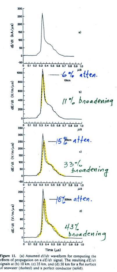
The three lower plots show the dE/dt signal at 10, 35, and 50 km range. The signals are both attenuated and broadened (the percentage refer to the pulse width at half maximum). The solid line shows propagation over a perfectly conducting surface for comparison (the dE/dt and dI/dt waveforms would be identical). Results from this calculation were used to correct measured dE/dt signals for attenuation caused by propagation.
And here are the main results from the experiment. First the estimate of peak I derived from measured E amplitudes using the transmission line model expression.
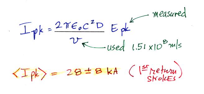
Note the value of the velocity used in the calculation is the the one that gave the best fit between measured I and E values in the experimental test of the transmission line discussed earlier in today's class.
Next the estimate of peak dI/dt
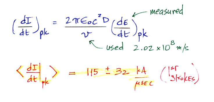
Again the velocity from
the experimental test of the
transmission line model was
used. Note the value used
for dI/dt is different from the
value used to estimate peak I.
We should remember that these estimates of peak I and peak dI/dt are for first return strokes in natural lightning. First return strokes do not occur in rocket triggered lightning. The peak I estimates are larger than the values summarized in our March 4 class which were for subsequent strokes in triggered lightning and lightning strikes to towers. The peak dI/dt values compare very well with the rocket triggered lightning measurements. My feeling is that the values above are some of the best estimates of peak I and peak dI/dt for first return strokes available.
Let's go back to our summary of the results of the experimental test of the transmission line model.
Much better agreement between transmission line model derived velocities and measured velocities was obtained when the Eshoulder amplitude was used instead of Epeak in the transmission line model equation together with Ipeak This is particularly true for the 1987 experiment with its simpler launch platform. Keep the 1.51 x 10⁸ m/s and the 2.02 x 10⁸ m/s velocity values in mind, we'll being referring to them again shortly in the final section in today's notes.
We should note that we still haven't explained why a different vTLM was obtained when using dE/dt and dI/dt data. The transmission line model can't account for this difference. There is another lightning return stroke current model, the so called Traveling Current Source model that does produce a difference like this. We may discuss that model briefly in a future lecture.
We'll end this lecture with a look at some experimental measurements of distant electric radiation fields and estimates of peak I and peak dI/dt values that were derived from them. The measurements are described in the publication cited below.
"Submicrosecond fields radiated during the onset of first return strokes in cloud-to-ground lightning," E.P. Krider, C. Leteinturier, and J.C. Willett, J. Geophys. Res., 101, 1589-1597, 1996.
Here are some important points regarding this experiment.
1. Electric fields from lightning first return strokes 25 to 45 km away were measured. Only the radiation field component is present at these ranges. Propagation between the strike point and the recording station was entirely over salt water so that high frequency signal content was largely preserved. The recording station was actually one of the stations used in the triggered lightning experiment described above (Point 2 on the map at the start of today's lecture)
2. The recording instrumentation was triggered on an RF signal rather than on E or dE/dt to prevent trigger bias.
The plot above shows range normalized dE/dt data versus range. A trigger threshold on an oscilloscope or waveform recorder, a fixed voltage, will correspond to larger and larger dE/dt values with increasing range. Between about 40 and 80 km the distribution of measured dE/dt signals will be biased toward larger signal amplitudes. Only the green points on the plot above which are above the trigger threshold would be recorded, beyond about 80 km very few of the dE/dt signals would be large enough to trigger the recording instrumentation. (This is a realistic but fictitious data set being used for illustration, both in the figure above and the histogram below).
The histograms below show the effect of trigger level bias on the distribution of range normalized dE/dt measurements. The first histogram plots the range normalized dE/dt measurements between 40 and 80 km which triggered the recording system. The mean value was 44 V/(m μsec).
The bottom histogram is the true distribution. I.e. it includes the data that triggered the recording system and those that did not. Including the latter group of data lowers the mean to 38 V/(m μsec).
The table below illustrates how measured dE/dt values can be range normalized.
3. Even though E field propagation was over salt water some high frequency attenuation was still present. An attempt was made to correct for this.
Here's one simple explanation of why the higher frequency signals are preferentially attenuated as they pass over a surface with finite conductivity.
Two signals with the same amplitude, but a factor of 2 difference in wavelength and frequency, are shown. The signals will cause charge to be induced on the surface. If we assume a voltage difference Δ V between locations of the + and - charge, currents will begin to flow in the ground. The current created by the signal with lower frequency will be a little smaller than the current created by the higher frequency signal. More power will be dissipated by the current created by the higher frequency signal than the lower frequency signal. This will reduce the amplitude of the higher frequency signal more than the lower frequency signal.
I'm not sure this approach is valid. Here's an alternate explanation.
Krider, Leteinturier, and Willett tried to determine the effects of propagation. The dI/dt waveform used in the calculations is shown at the top of the figure below.
The three lower plots show the dE/dt signal at 10, 35, and 50 km range. The signals are both attenuated and broadened (the percentage refer to the pulse width at half maximum). The solid line shows propagation over a perfectly conducting surface for comparison (the dE/dt and dI/dt waveforms would be identical). Results from this calculation were used to correct measured dE/dt signals for attenuation caused by propagation.
And here are the main results from the experiment. First the estimate of peak I derived from measured E amplitudes using the transmission line model expression.
Note the value of the velocity used in the calculation is the the one that gave the best fit between measured I and E values in the experimental test of the transmission line discussed earlier in today's class.
Next the estimate of peak dI/dt
We should remember that these estimates of peak I and peak dI/dt are for first return strokes in natural lightning. First return strokes do not occur in rocket triggered lightning. The peak I estimates are larger than the values summarized in our March 4 class which were for subsequent strokes in triggered lightning and lightning strikes to towers. The peak dI/dt values compare very well with the rocket triggered lightning measurements. My feeling is that the values above are some of the best estimates of peak I and peak dI/dt for first return strokes available.