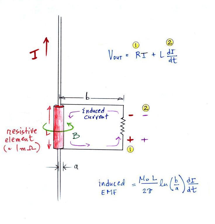
Ideally the voltage across the
"shunt" would be R times I (R is the resistance of the shunt
and I is the lightning current). Very low resistance
values (on the order of a milliohm) are needed because peak
lightning current amplitudes are large.
As the picture above shows however, measuring the voltage across the shunt introduces a loop circuit. The lightning will produce a time varying magnetic field that will couple into the loop. This will add an L dI/dt term to the output voltage. Even if L is small, the lightning peak dI/dt can be very large.
The problem with induced voltages in the measuring circuit can be avoided if a coaxial shunt design is used.
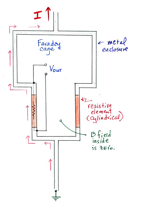
Here's a crossectional view. The resistive element has a cylindrical shape and the measuring circuit is inside the cylinder where the magnetic field is zero (B fields from currents flowing in the right and left hand sides of the cylinder point in opposite directions and cancel). The measuring instrumentation is placed in the metal enclosure (rectangular or cylindrical), a Faraday cage, at the top part of the figure. Signals could then be sent out on fiber optics cables to a nearby trailer for recording. Current is shown flowing through one side of the diagram. In reality it flows through all sides.
There can still be some problems with a coaxial shunt. Large currents can heat the resistive element and change the resistance (or heat it so much that it is damaged). Also high frequency currents may only flow through the skin and not through the entire volume of the resistive element and the actual resistance wouldn't be known.
A schematic illustration from one of the triggered lightning experiments in Florida (at the northern edge of the Kennedy Space Center in this case, not at the Univ. of Florida site. Source: Leteinturier, C., J.H. Hamelin, A. Eybert-Berard, "Submicrosecond Characteristics of Lightning Return-Stroke Currents," IEEE Trans. EMC, 33, 351-357, 1991).
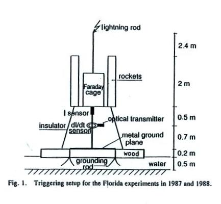
A coaxial shunt (I sensor in the figure) was positioned just below the Faraday cage (which contained the measuring equipment and also the electronics that controlled firing of the rockets). A dI/dt sensor surrounds the lightning current conductor a little bit further down. This launch platform was actually floating on brackish water.
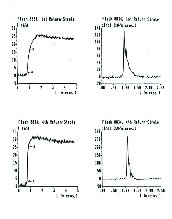
The next figure shows some examples of lightning I and dI/dt records from two strokes in a flash triggered during the 1988 experiments in Florida (the experiments were at the Kennedy Space Center, not at the Gainesville site mentioned in the last class).
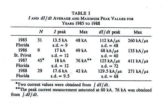
This first figure gives mean peak I and peak dI/dt values from rocket triggered lightning experiments conducted in Florida (at the Kennedy Space Center) and at the Saint Privat d'Allier station in central France (where the rocket triggered lightning experiments were first conducted). With the exception of the 1986 St. Privat dI/dt data (where there appears to have been a shielding problem with the dI/dt sensor), the mean values from the different summer field experiments are generally in pretty good agreement. The overall average peak I value is 16.6 kA and the average peak dI/dt value (France 1986 data omitted) is 122 kA/μs. Remember that return strokes in triggered lightning are thought to be comparable to subsequent return strokes in natural lightning.
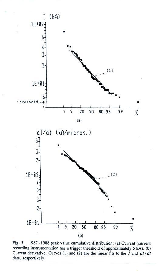
Lightning current parameters such as peak I and peak dI/dt are often log-normally distributed. Data that are log-normally distributed should fall in a straight line on a cumulative probability plot. Cumulative probability distributions of peak I and peak dI/dt from the Florida 1987 and 1998 experiments are shown below.
As the picture above shows however, measuring the voltage across the shunt introduces a loop circuit. The lightning will produce a time varying magnetic field that will couple into the loop. This will add an L dI/dt term to the output voltage. Even if L is small, the lightning peak dI/dt can be very large.
The problem with induced voltages in the measuring circuit can be avoided if a coaxial shunt design is used.
Here's a crossectional view. The resistive element has a cylindrical shape and the measuring circuit is inside the cylinder where the magnetic field is zero (B fields from currents flowing in the right and left hand sides of the cylinder point in opposite directions and cancel). The measuring instrumentation is placed in the metal enclosure (rectangular or cylindrical), a Faraday cage, at the top part of the figure. Signals could then be sent out on fiber optics cables to a nearby trailer for recording. Current is shown flowing through one side of the diagram. In reality it flows through all sides.
There can still be some problems with a coaxial shunt. Large currents can heat the resistive element and change the resistance (or heat it so much that it is damaged). Also high frequency currents may only flow through the skin and not through the entire volume of the resistive element and the actual resistance wouldn't be known.
A schematic illustration from one of the triggered lightning experiments in Florida (at the northern edge of the Kennedy Space Center in this case, not at the Univ. of Florida site. Source: Leteinturier, C., J.H. Hamelin, A. Eybert-Berard, "Submicrosecond Characteristics of Lightning Return-Stroke Currents," IEEE Trans. EMC, 33, 351-357, 1991).
A coaxial shunt (I sensor in the figure) was positioned just below the Faraday cage (which contained the measuring equipment and also the electronics that controlled firing of the rockets). A dI/dt sensor surrounds the lightning current conductor a little bit further down. This launch platform was actually floating on brackish water.
The next figure shows some examples of lightning I and dI/dt records from two strokes in a flash triggered during the 1988 experiments in Florida (the experiments were at the Kennedy Space Center, not at the Gainesville site mentioned in the last class).
We'll finish this
portion of the topic with a quick look at some of
the results from some of the triggered lightning
experiments and then compare those results with
data from some of the older lightning current
measurements during lightning strikes to
instrumented towers made in Switzerland and
Italy.
This first figure gives mean peak I and peak dI/dt values from rocket triggered lightning experiments conducted in Florida (at the Kennedy Space Center) and at the Saint Privat d'Allier station in central France (where the rocket triggered lightning experiments were first conducted). With the exception of the 1986 St. Privat dI/dt data (where there appears to have been a shielding problem with the dI/dt sensor), the mean values from the different summer field experiments are generally in pretty good agreement. The overall average peak I value is 16.6 kA and the average peak dI/dt value (France 1986 data omitted) is 122 kA/μs. Remember that return strokes in triggered lightning are thought to be comparable to subsequent return strokes in natural lightning.
Lightning current parameters such as peak I and peak dI/dt are often log-normally distributed. Data that are log-normally distributed should fall in a straight line on a cumulative probability plot. Cumulative probability distributions of peak I and peak dI/dt from the Florida 1987 and 1998 experiments are shown below.
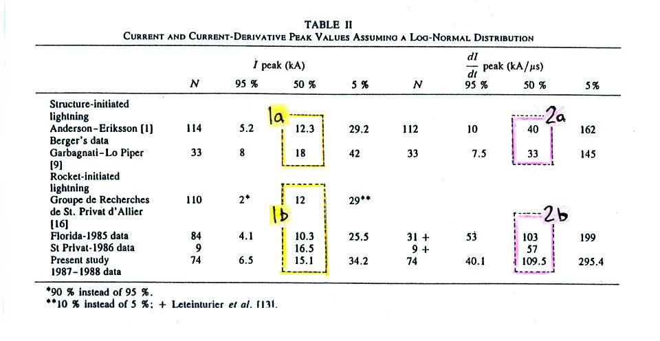
Parameters from
these distributions are summarized in the table
below together with parameters from the Swiss and
Italian tower measurements.
Generally the 50%
values (the median) of peak I from the tower
measurements (1a) compare very well with the peak
I values from the rocket triggered lightning
experiments (1b).
The sensors and recording equipment used for the tower measurements in Switzerland and Italy probably didn't have fast enough time resolution to accurately measure peak dI/dt values. The data in the table above seem to reflect this. The tower derived measurements (2a): 40 and 33 kA/μs are significantly lower than the values obtained during the triggered lightning experiments (2b): 103 and 109.5 kA/μs (we disregard the 57 kA/μs value from the St. Privat 1986 campaign).
We will note that indirect estimates of peak return stroke dI/dt derived from remote measurements of radiated fields, which will be the subject of our next lecture, agree well with direct measurements in rocket triggered lightning.
In this lecture we will learn how lightning return stroke current parameters such as Ipk and (dI/dt)pk might be estimated from remote measurements of E and B fields. It is much easier to make remote measurements of lightning electric and magnetic fields than it is to make direct measurements of lightning return stroke currents. There is no first return stroke in a rocket triggered cloud-to-ground discharge, just return strokes. We can hope to learn something about peak I and dI/dt in first return strokes when we use E and B field measurements.
Radiated Fields
We must first learn more about the fields radiated by lightning.
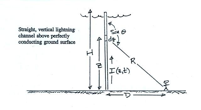
First here's the geometry used in the E and B fields calculations that follow. The lightning channel is assumed to be straight and vertically oriented. The ground is flat and a perfect conductor. Just as we used the method of images problem earlier in the semester to solve a problem in electrostatics, we can match the boundary condition at the ground surface by replacing it with an image of the lightning channel below the ground.
In a problem of this kind you are basically trying to find E and B that satisfy Maxwell's equations.
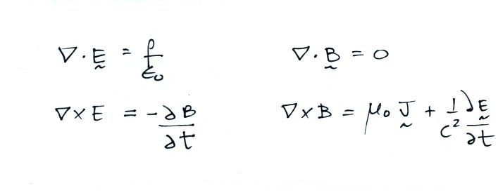
The general approach is to find the scalar and
vector potentials φ and A
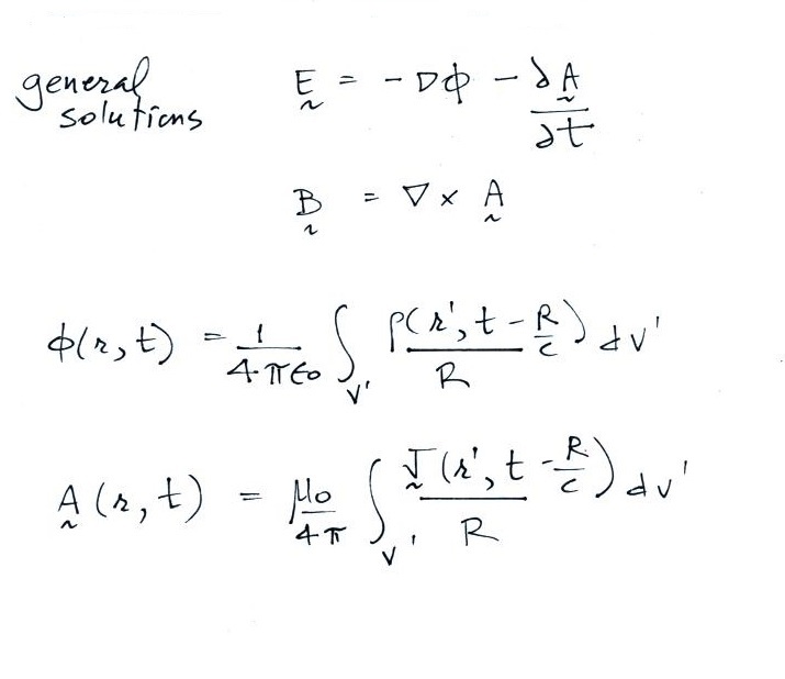
We aren't going to look at all the steps in the derivation, we'll simply write down the results. If you are interested in the details a good place to start would be the following article: "The Electromagnetic Radiation from a Finite Antenna," M.A. Uman, D.K. McLain, and E.P. Krider, Am. J. Phys., 43 33-38, 1975.
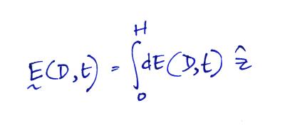
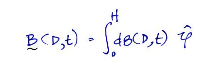
To obtain the total E field we need to integrate from the ground to the top of the channel
At the ground the magnetic field has just an azimuthal component
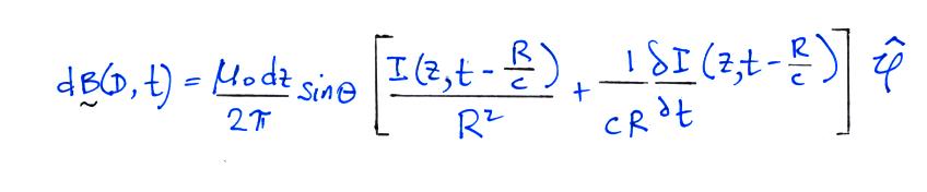
and again we integrate over the length of the channel to determine the total field.
I should mention also that a recent publication points out and corrects a small error in the expressions above. This won't affect our discussion, but if you would like to see the correct expressions, click here.
Static, Induction, and Radiation field terms
We won't really be using these rather complex general expressions. Rather let's just note that the electric field expression contains terms involving a time integral of current, the current itself, and a time derivative term.
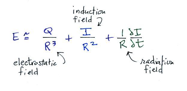
We refer to these are the electrostatic, induction, and radiation field components. The B field has just induction and radiation field components.
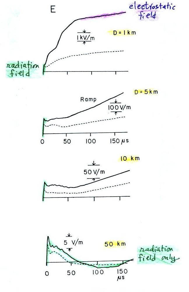
Except for the very beginning of the discharge, the electrostatic field is generally dominant at close range. Because it decreases as 1/R, the radiation field is the only field component observed at long range (beyond a few 10s of kilometers). Also because peak dI/dt occurs very early in a return stroke discharge, the radiation field also dominates at the very beginning of a return stroke.
The sketch below provides a rough idea of the what the 3 field components would look like given the current waveform at the top of the figure.
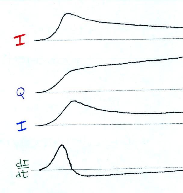
The solid lines show typical first return field
values, the dotted lines are for subsequent
strokes. These aren't actual
waveforms. Rather they are essentially an
average of measurements of actual waveforms (lots
of waveforms).
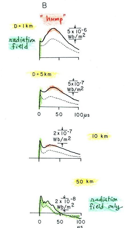
The hump on these magnetic fields is probably coming from the induction field. We don't see it on E field waveforms because the electrostatic field component dominates. B fields don't have a magnetostatic field component.
The sensors and recording equipment used for the tower measurements in Switzerland and Italy probably didn't have fast enough time resolution to accurately measure peak dI/dt values. The data in the table above seem to reflect this. The tower derived measurements (2a): 40 and 33 kA/μs are significantly lower than the values obtained during the triggered lightning experiments (2b): 103 and 109.5 kA/μs (we disregard the 57 kA/μs value from the St. Privat 1986 campaign).
We will note that indirect estimates of peak return stroke dI/dt derived from remote measurements of radiated fields, which will be the subject of our next lecture, agree well with direct measurements in rocket triggered lightning.
In this lecture we will learn how lightning return stroke current parameters such as Ipk and (dI/dt)pk might be estimated from remote measurements of E and B fields. It is much easier to make remote measurements of lightning electric and magnetic fields than it is to make direct measurements of lightning return stroke currents. There is no first return stroke in a rocket triggered cloud-to-ground discharge, just return strokes. We can hope to learn something about peak I and dI/dt in first return strokes when we use E and B field measurements.
Radiated Fields
We must first learn more about the fields radiated by lightning.
First here's the geometry used in the E and B fields calculations that follow. The lightning channel is assumed to be straight and vertically oriented. The ground is flat and a perfect conductor. Just as we used the method of images problem earlier in the semester to solve a problem in electrostatics, we can match the boundary condition at the ground surface by replacing it with an image of the lightning channel below the ground.
In a problem of this kind you are basically trying to find E and B that satisfy Maxwell's equations.
We aren't going to look at all the steps in the derivation, we'll simply write down the results. If you are interested in the details a good place to start would be the following article: "The Electromagnetic Radiation from a Finite Antenna," M.A. Uman, D.K. McLain, and E.P. Krider, Am. J. Phys., 43 33-38, 1975.
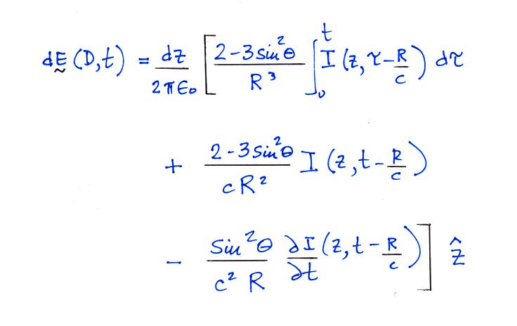
The expression below gives
the electric field radiated by a short segment
dz located at an altitude z above the
ground. We'll limit our attention to the
E field at the ground (assumed to be a perfect
conductor) which has just a z component.
There is interest in how lightning E and B
fields couple onto electric power lines.
To properly examine this problem you would
need to compute E and B for points above the
ground (at the level of the power
lines). That becomes a more complicated
problem because the E and B fields will each
have 3 components (vertical, radial, and
azimuthal components in cylindrical geometry).
To obtain the total E field we need to integrate from the ground to the top of the channel
At the ground the magnetic field has just an azimuthal component
and again we integrate over the length of the channel to determine the total field.
I should mention also that a recent publication points out and corrects a small error in the expressions above. This won't affect our discussion, but if you would like to see the correct expressions, click here.
Static, Induction, and Radiation field terms
We won't really be using these rather complex general expressions. Rather let's just note that the electric field expression contains terms involving a time integral of current, the current itself, and a time derivative term.
We refer to these are the electrostatic, induction, and radiation field components. The B field has just induction and radiation field components.
Except for the very beginning of the discharge, the electrostatic field is generally dominant at close range. Because it decreases as 1/R, the radiation field is the only field component observed at long range (beyond a few 10s of kilometers). Also because peak dI/dt occurs very early in a return stroke discharge, the radiation field also dominates at the very beginning of a return stroke.
The sketch below provides a rough idea of the what the 3 field components would look like given the current waveform at the top of the figure.
More realistic
shapes of the E and B waveforms that you might
expect to see at various distances from a CG
stroke are shown below (source: Lin,
Y.T.,
M.A.
Uman,
J.A.
Tiller,
R.D.
Brantley,
W.H. Beasley, E.P. Krider, C.D. Weidman,
"Characterization of Lightning Return Stroke
Electric and Magnetic Fields from
Simultaneous Two-Station Measurements," J.
Geophys. Res., 84-6307-6314, 1979).
.
.
The hump on these magnetic fields is probably coming from the induction field. We don't see it on E field waveforms because the electrostatic field component dominates. B fields don't have a magnetostatic field component.