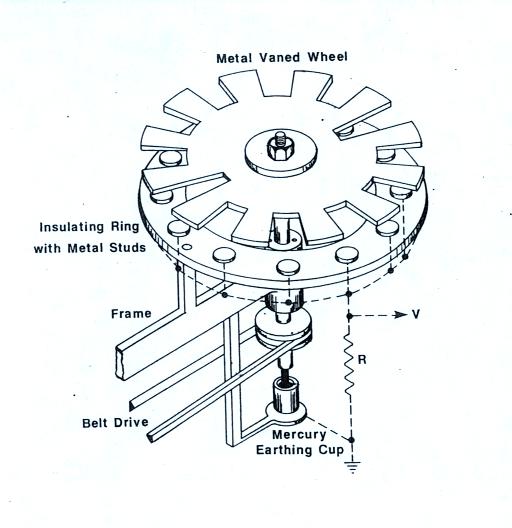
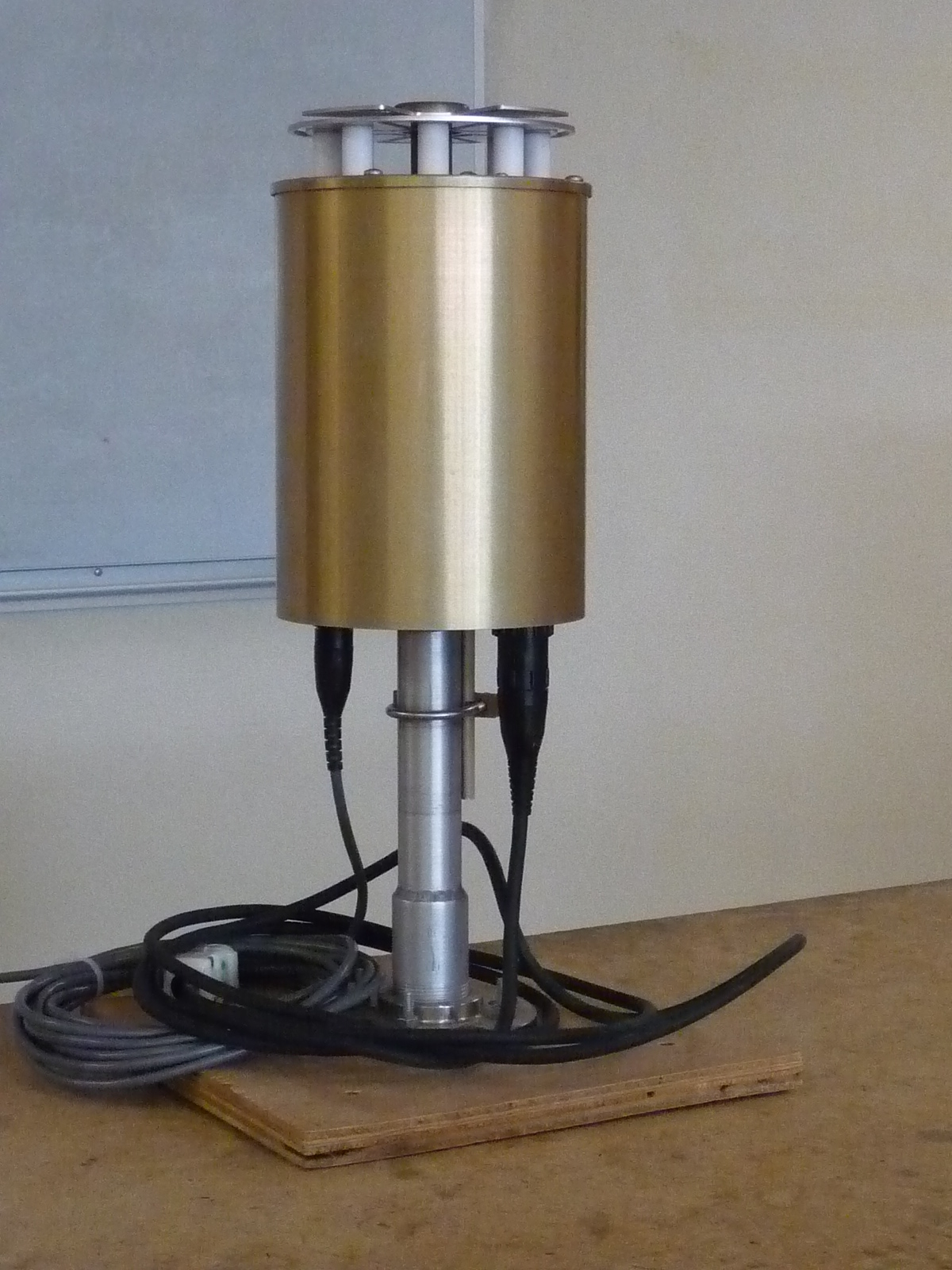
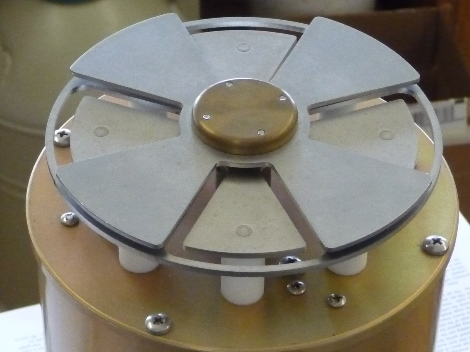
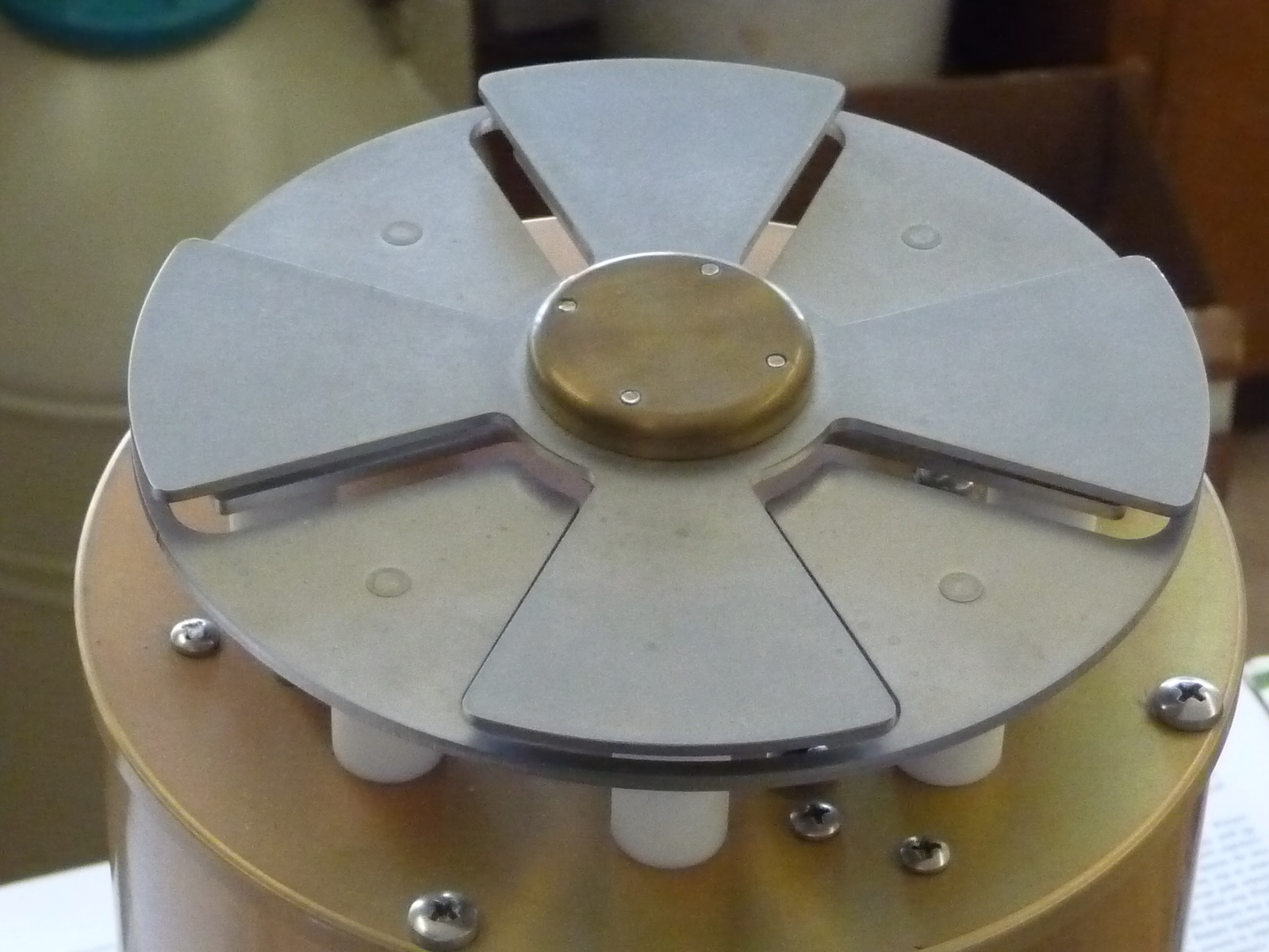
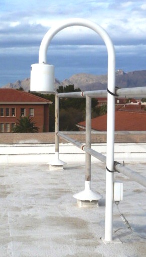
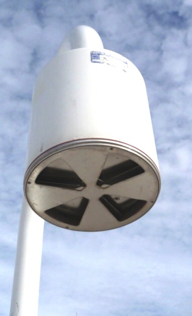
Monday Jan. 26, 2015

The first homework assignment of the semester was handed out today.  The assignment is due in 1 week, on Monday Feb. 2.  There will most likely be a second assignment handed out on Friday (you'll have a week to complete that assignment also). 

We finished class last Friday with the integral form of Gauss' Law


The surface integral of electric field over a surface enclosing a charge q is just q divided by εo the integral form of Gauss' Law.  The shape of the surface is irrelevant.

Infinite line charge revisited
To see how useful this expression can be we'll return to our earlier problem involving the infinitely long uniform line of charge and use Gauss' Law to determine the electric field.  We'll see that it is a much easier process this time around.


The crucial part of the problem is the choice of surface.  We draw a cylinder centered on the line of charge.  This is the area that we will integrate E over in the Gauss Law expression.  It is also important to realize that the E field has a radial component only.


There is no contribution to the surface integral from the ends of the cylinder (E is perpendicular to the normal vector, the dot product between E and n is therefore zero).  E is parallel to the normal vector along the side of the cylinder.  E is also constant on the side of the cylinder (E is a function of r and r stays constant as you integrate over the surface of the cylinder side).  In the end we obtain the same expression for E as we did in the example worked out last week.


It's relatively easy to show that the surface integral of the E is zero when charge is located outside the volume.  We didn't work through this example in class.


This might be a little hard to visualize because the figure isn't drawn very well.  But along the front portion of the surface the r unit vector points inward, n points outward.  Along the back surface r and n both point outward.  The two increments of solid angle have the same value but opposite signs so they cancel.  We've only shown part of the entire surface.  But as you move over the rest of the surface there will always be a surface element in the front and in the back and the two contributions will cancel each other out.


Gauss' Law (differential form)
We'll go back to the integral form of Gauss' Law.


A surface S contains a volume V.  We can use the divergence theorem to write the surface integral of electric field as a volume integral of the divergence of the electric field.  The charge enclosed by the surface is just the volume integral of the volume charge density.  Combining these two expressions


In order for the two volume integrals to be equal for an arbitrary volume, the terms inside the integrals must be identical.


E field inside a conductor


Free electrons inside the conductor will quickly move around and redistribute themselves in such a way that they will cancel out the field in the conductor (as the electrons move they leave behind positively charged atoms).  Very quickly the field inside the conductor will become zero.  There is also no space charge inside the conductor, all the charge is distributed along the surface on the conductor.  The electric field lines in the vicinity of the conductor will be distorted and will strike the surface of the conductor perpendicular (if there were any tangential component, charges would move and cancel it out).

E field and surface charge density at the surface of a conductor
Next we'll use Gauss' Law to determine a relationship between the surface charge density and the electric field strength at the surface of a conductor.

A cylindrical volume, half inside and half outside the conductor is used.  You must integrate the electric field, E, over the surface of the cylinder. 

1.  The E field is zero inside the conductor.  So you get no contribution to the surface integral from the bottom end of the cylinder.


2.   Both the sides of the cylinder and the E field lines are perpendicular to the surface of the conductor.  The dot product of E and the normal to the cylinder surface is zero (E and n are perpendicular)  So there is no contribution to the surface integral from the sides of the cylinder.

3.   The only contribution comes from the top end of the cylinder.  E and the normal vector are parallel.  So the contribution from the top end is just E A, where A is the area of the top end of the cylinder.   The charge enclosed is just A σ, where σ is the surface charge density.  The electric field at the surface of the conductor is perpendicular to the conductor and has the value highlighted in yellow.


We plugged a value for the fair weather electric field into this expression on the first day of class to determine the charge density on the surface of the earth.


I had originally planned to introduce the electrostatic potential at this point.  But there wouldn't have been enough time for the next section on electric field mills.  So I've moved the material on electrostatic potential to the Wednesday, Jan. 28 class notes.


Now some applications of what we have been learning.  In this and the next class we'll looking at a couple of instruments used to measure thunderstorm and lightning electric fields. 

Electric field mill
The first is an electric field mill used to measure static and slowly time varying electric fields.  Referring to the figure below at left (from Uman's 1987 The Lightning Discharge book).  The sensors (referred to as studs in the figure) are covered by a rotating grounded plate.  The rotating plate is notched or slotted so that the sensors are periodically exposed to and covered (shielded) from the ambient electric field.  A photograph of the field mill shown in class is shown below at right (signal and power cables are connected at the bottom of the mill).


The two photographs below are closeups of the top of the field mill


The stator plates are exposed to the E field at left and covered in the photograph at right.  The four stators (sensor plates) exposed in the figure at left are connected together electrically.  Another four stators, also connected together are exposed in the figure at right.  Thus this field mill has two sets of sensors.  One set is exposed while the other set is covered.  This just makes it possible to make measurements of the E field two times more often.

The next figure shows currents flowing into and out of the sensor plate in response to an incident E field.


The sensor plate is covered at Point 1.  At Point 2 the sensor is uncovered and we assume the ambient field points upward (toward negative charge in the lower part of a thunderstorm perhaps).  Positive charge flows up to the sensor plate.  The current flows from the sensor in Point 3 because the sensor has been covered and shielded from the E field.  Points 4 and 5 are similar except the polarity of the E field has been changed. 

Note the current signals at Points 2 & 5 are the same even though the field polarities are reversed.  You must keep track of when the sensor is covered and uncovered in order to determine the polarity of the incident E field.

It is a relatively simple matter to relate the amplitude of the signal current to the intensity of the incident E field.


We use the expression derived a few days ago relating the E field at the surface of a conductor and the surface charge density (sigma in the equations above).  A is the area of the sensor.

If you integrate the current (connect the sensor through a capacitor to ground) you obtain an output voltage that is proportional to E.


We were able to electrify a couple of objects using triboelectric charging (see the handout from class on Wed., Jan. 21).  For example rubbing a piece of PVC pipe with cat or rabbit's fur should charge the pipe negatively.  We were able to verify when the charged piece of pipe was held above the field mill and we saw a negative polarity output signal.    Rubbing a glass graduated cylinder with the same piece of fur charged the glass positively. 

We were also able to confirm that the dome on the Van de Graaff generator was indeed negatively charged as mentioned in last Wednesday's class (the newer Van de Graaff generator was positively charged).

Another electric field mill was also shown (but not operated) in class.  This particular instrument was designed and built by a local company Mission Instruments Corporation.


Inverted field mill
close up of the field mill sensor plate

The field mill is shown bolted to a railing on the roof of the PAS building here on campus.  One reason for inverting the field mill is so that charged precipitation won't fall on the sensor plate and introduce a spurious noise signal.  The E field will be distorted by the metal mast and the field mill would need to be calibrated against a second mill placed nearby but mounted flush with the ground surface.  In the situation above the building and railing would also distort the E field.  We'll look at E field enhancement in a day or two.


Next we looked at an example of an E field record obtained with an electric field mill.  The data come from the Kennedy Space Center field mill network.

The first record is interesting because it shows the transition from fair to foul or stormy weather electric fields (a change in polarity and in field strength).


At the very beginning of the fields were about +200 V/m.  The field crosses zero at about 20:39:00 GMT and increases in amplitude, eventually reaching about -2500 V/m.  The abrupt transitions are caused by lightning.  In our next lecture we will expand the time scale and look at the field variations that occur in an individual discharge.  Later in the course we'll come back to field records like this and show what we start to learn something about the locations of charge and amounts of charge involved in lightning discharges by analyzing the electric field changes at multiple locations.

Note that we referred to a positive 200 V/m fair weather electric field even though the field was pointing downward toward negative charge on the ground.  The vertical axis in the figure above is labeled potential gradient rather than electric field.  This brings up a confusing situation regarding electric field polarities that you should be aware of; something that might cause some confusion if you ever read through the atmospheric electricity literature.


The figure above at left correctly show the E field pointing downward toward negative charge on the earth's surface during fair weather.  The E field reverses direction under a thunderstorm.  The main negative charge center in the cloud causes positive charge to build up in the ground under the storm.  The E field points upward.

A physicist would consider the fair weather field to be negative polarity because it points downward and would call the stormy weather field positive.  The atmospheric electricity community will often refer to the fair weather field as positive and would call the foul weather field negative.  This can be a source of confusion. 

Because the electric field and the potential gradient have opposite signs


atmospheric electricians can refer to the positive amplitude signal they are used to seeing during fair weather as a positive potential gradient rather than a positive electric field.  That is consistent with the physics sign convention.  A positive 200 V/m potential gradient is equal to a -200 V/m electric field and everyone is happy.