Wednesday, Jan. 28, 2015
Electrostatic potential
We'll start with something we weren't able to cover in class on
Monday - electrostatic potential.
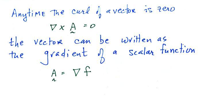
I'm not enough of a mathematician to be able to explain why
this is true (other than demonstrating that the curl of a gradient
is zero). We'll just have to accept that on faith. And
actually figuring out what the scalar function needs to be is
another problem.
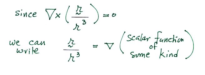
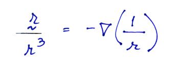
The curl of the r (a vector) over r3
(magnitude of r cubed) term in the expression for electric field
is zero.
The scalar function in this case is - (1/r)
We'll insert this into the
expression for electric field.
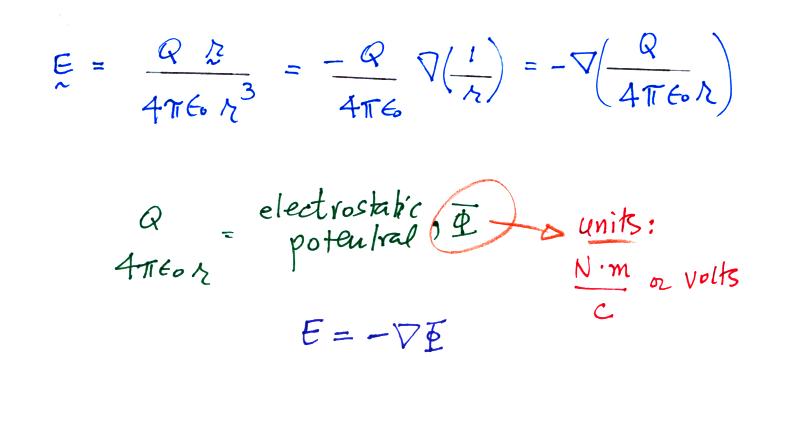
It is often much simpler to determine the electrostatic
potential because it is a scalar quantity. The electric
field can then be determined by taking the gradient of the
potential.
We
didn't cover any of this short digression in class.
When the curl of a vector field is zero, the vector field
is irrotational. There's a pretty good online
animation that shows both irrotational and
rotational vortices (spinning fluids).
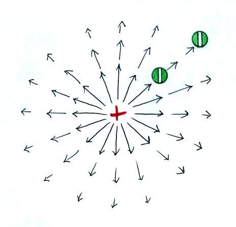
The pattern of electric field vectors around a positive
charge would look something like the figure below.
We can imagine that the arrows represent fluid motion and
can picture what would happen if a small object were
placed in the moving fluid (as was done in the animation
above). It would move outward without any rotation.
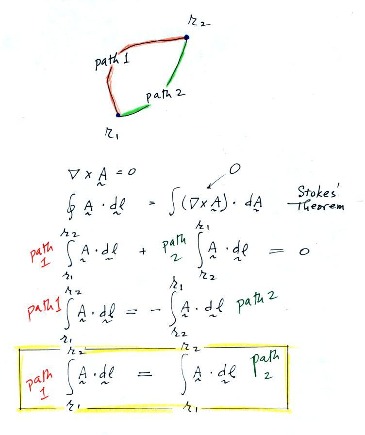
An irrotational field has another important
property. A line integral from from one point to
another will be independent of the integration path.
Because the curl is zero we can use Stokes' Theorem to say
the line integral of the vector around a closed loop is
also zero. The rest of the argument follows fairly
simply from that.
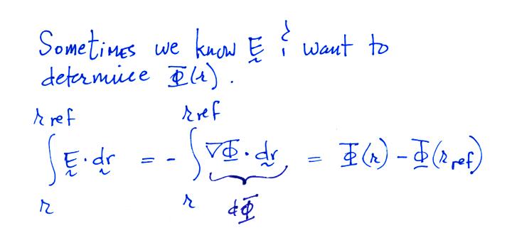
Sometimes rather than starting with Φ and
then determining the E field, we might know the E field
and want to determine Φ.
We can determine the
potential as shown above (there's no reason rref
needs to be the upper limit, it could just as easily be
the lower limit)
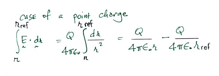
Let's assume a point charge and substitute in an
expression for E into the left integral above.
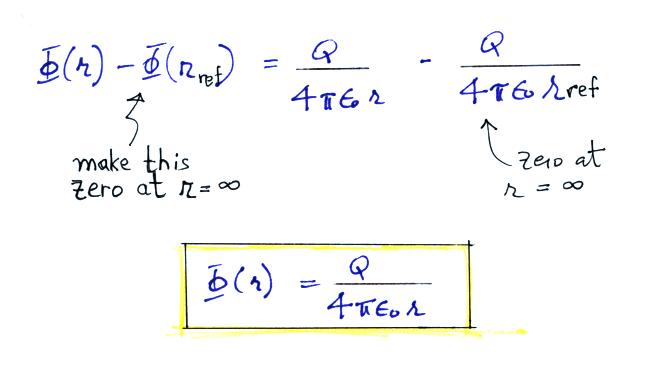
We'll set this equal to the earlier expression
We get our earlier result (provided we assume that Φ(r = ∞)
is zero)
We can write the electric
field as the gradient of the electrostatic potential and
then substitute that into Gauss' Law.
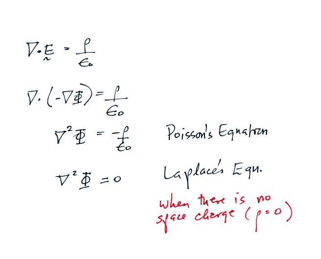
We obtain Poisson's Equation. Laplace's equation
applies in situations where the volume space charge
density is zero. We'll be using Laplace's equation
in our next lecture. Here is a handout
with vector differential operators (Laplacian, curl,
gradient and divergence) in cartesian, cylindrical, and
spherical coordinate systems.
"Fast" and "slow" E field antenna systems
Another example of a field mill record, one hour of actual
thunderstorm and lightning fields recorded at the Kennedy Space
Center, is shown below (from: Livingston and Krider (1978)).
The abrupt transitions are caused by lightning and are
superimposed on a static field of about 3 kV/m (negative
potential gradient corresponds to a positive E field pointing
upward toward negative charge in the bottom of a
thunderstorm).
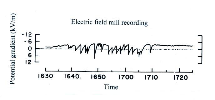
A field mill can be used to determine when
a thunderstorm becomes electrified and monitor electrical
activity in a thunderstorm. Note that a
fairly large dynamic range is needed (-12 kV/m to +12 kV/m) is
needed to insure that the E field remains on scale.
Later in the semester we will see that measurements of the
lightning field changes at multiple locations can be used to
determine the magnitude and location of the charge neutralized
by the lightning discharge.
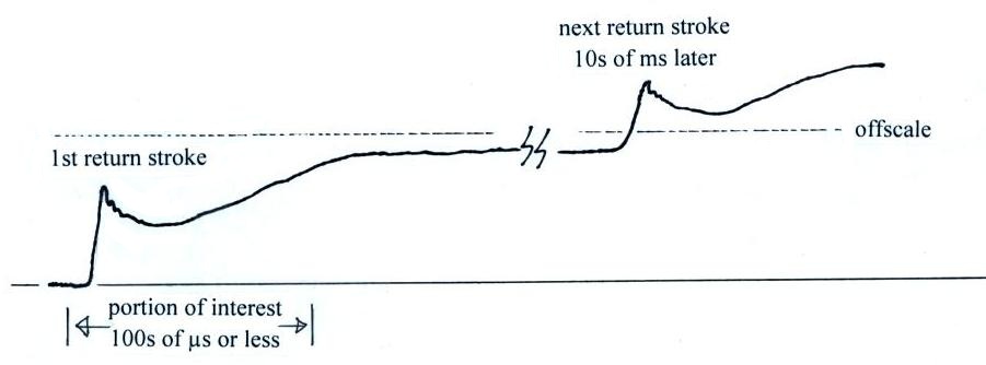
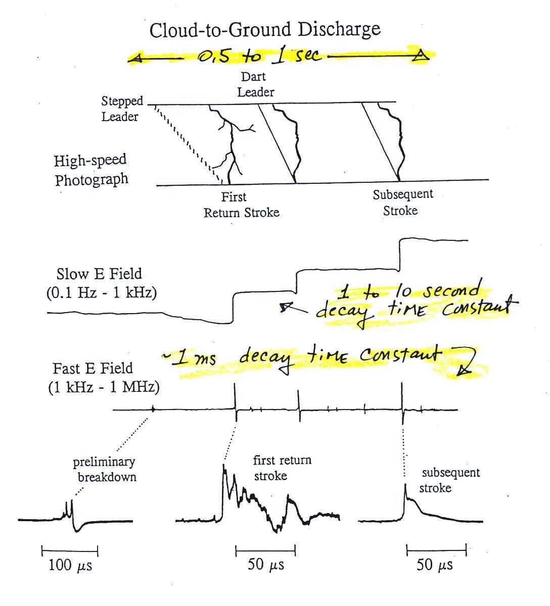
A lightning discharge only lasts 1 second or so and appears as
just an abrupt field change on the record above. We're going
to find that a lightning discharge consists of a series of
different processes that occur on millisecond, microsecond and
even sub microsecond time scales. The figure below
illustrates this (don't worry about all the details and names at
this point, we'll come back to this later in the semester).
An electric field mill can measure static and slowly varying
fields but wouldn't faithfully resolve all the field changes and
variations that occur on these faster time scales. We
need a different kind of measuring system.
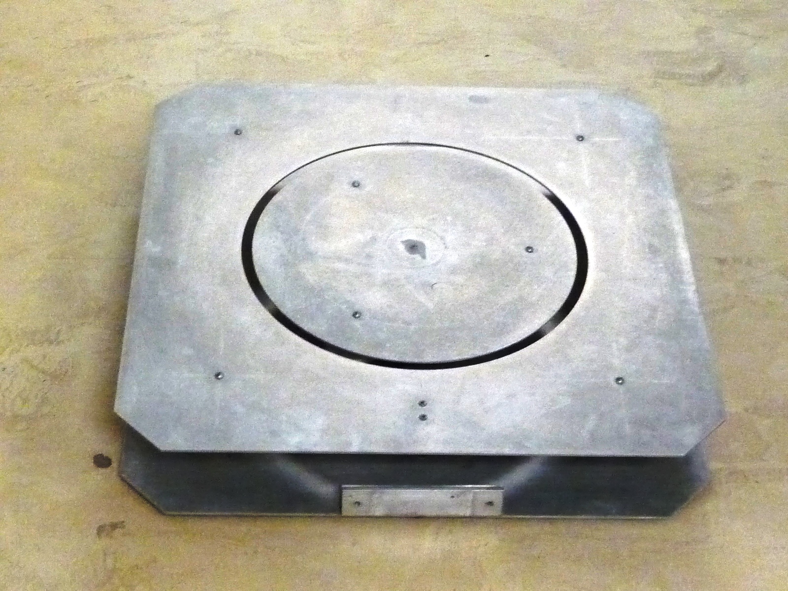
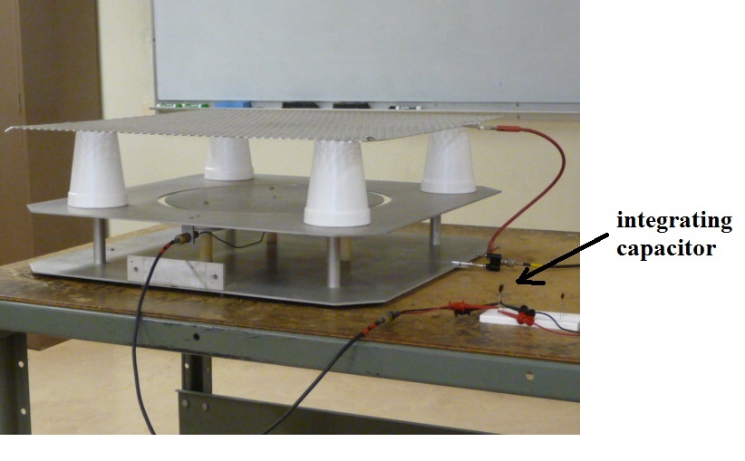
One way of measuring these faster time varying electric
fields is to use a flat plate antenna (aka flush plate dipole
antenna). It basically consists of a large flat grounded
plate that would be positioned on the ground (preferably flush
with the surrounding ground). A smaller circular insulated
sensor plate is found inside a center hole as shown in the
photograph below (the antenna is on the classroom floor in this
photograph). The center plate "senses" the
electric field and is insulated from ground.
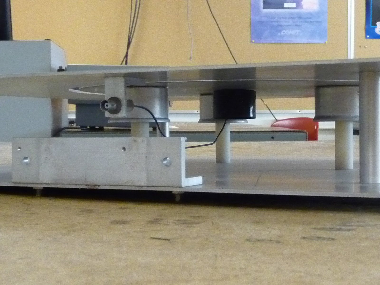
We look under the top plate of the antenna in the next picture.
The center sensor plate is supported by insulating nylon or Teflon
spacers. The top end of the supports are covered with "rain
hats" to try to keep the insulators dry during rainy
weather. A wire connection to the center plate connects to a
coaxial cable to carry the signal to processing and recording
equipment.
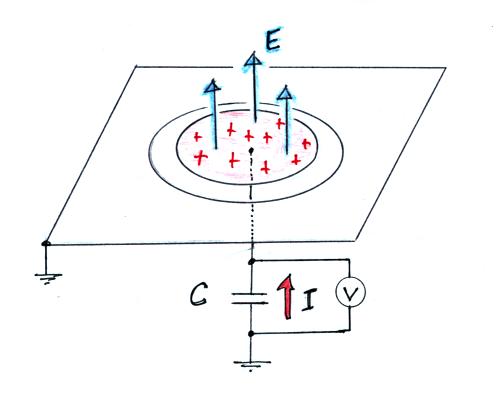
In some ways the operation of this antenna is similar to the field
mill. In this case a time varying E field causes current to
flow to and from the center sensor plate (you don't need to
repeatedly cover and uncover the sensor plate).
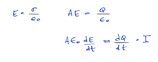
This current is proportional to the time derivative of the
electric field (σ in the
equation below is the surface charge density on the sensor
plate).
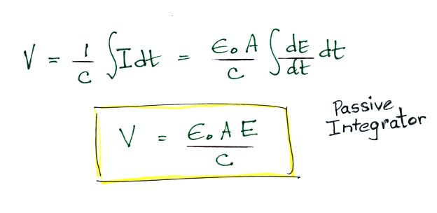
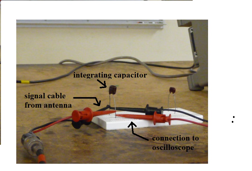
Integrating the current gives an output signal that is
proportional to E.
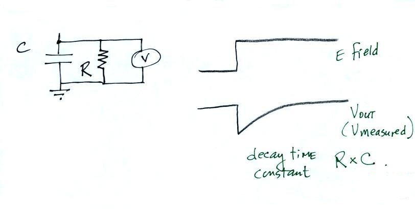
In the circuit above the antenna is connected to a capacitor, this
is a passive integrator. Some kind of measuring device would
then be connected across the capacitor.
The value of the RC decay time constant determines whether the
antenna works as a "slow" or a "fast" antenna system.
A Slow E field system with a long, 1 to 10 second
decay time would be appropriate if you wanted to study an
entire lightning discharge on a faster time scale. A
couple of actual Slow E field records are shown below (also
from the Livingston and Krider (1978) paper cited earlier).
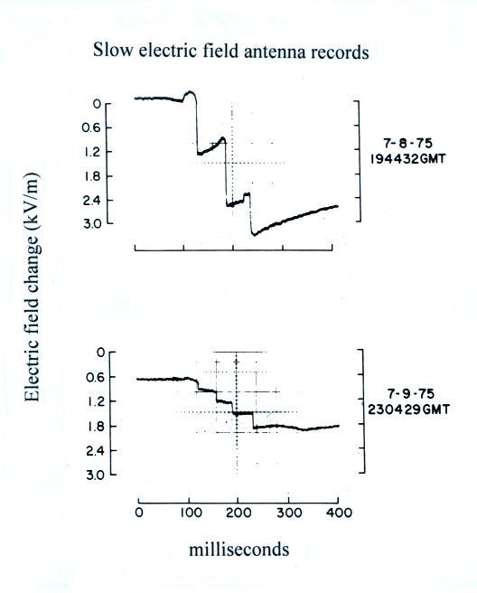
Note first the much faster time scale, 0.4
seconds full scale in this case. The step changes in the
E field are lightning strokes to the ground. The top
example shows a 3 stroke cloud-to-ground discharge. The
second discharge has 4 strikes to ground.
Because the Slow E antenna system does not have DC response
the static E field (which can be several kV/m) is effectively
filtered out (like switching from DC to AC coupling on an
oscilloscope). Lightning field changes can be examined
with more gain. Because the signals of interest last
from 0.5 to 1 second, a decay time constant of 10 seconds
would be appropriate here. The slow E field
would decay back to zero during the interval between lightning
discharges.
To give you some appreciation for how recording methods
have changed, the signals above were (I believe) displayed on
a storage oscilloscope and photographed with a Polaroid film
camera!
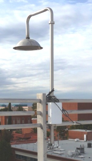
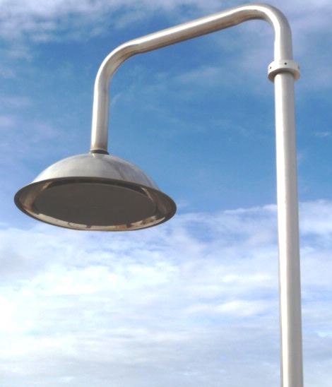
Because of the long decay time constant, charged
precipitation falling on a Slow E field antenna can drive the
signal off scale. Inverted antennas are sometimes used
to avoid that problem.
This antenna is mounted on the roof of the Penthouse atop
the PAS Building. Because of its exposed position and
the chance that it could be struck by lightning, signals are
brought into the Penthouse on a fiber optic cable.
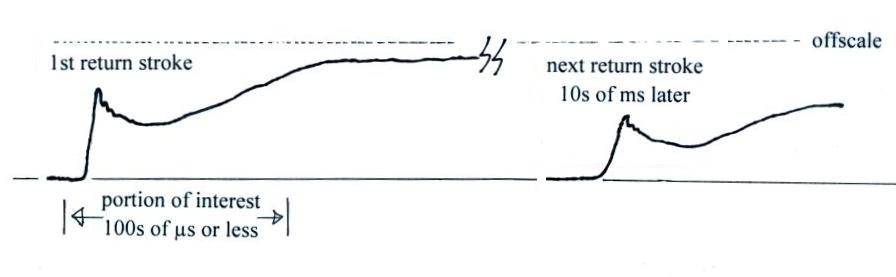
The E field variations that occur during a
individual return stroke could be examined by increasing the
vertical gain and displaying the Slow E field signals on a
faster time scale. However, as sketched below, the long
time decay would mean the signal might not decay back to zero
in the interval between return strokes.
A slow E field record (a few
seconds long decay time constant) displayed on a much faster
time scale.
The solution is to shorten the RC decay time constant.
This turns the slow antenna into a fast antenna system.
Same antenna but with a much shorter (milliseconds long) decay
time constant.
A decay time of about 1 to 10 milliseconds would be long
enough to accurately record the Fast E field variations but
would allow the signal to decay back to zero in the interval
between strokes. A short decay time constant would also mean
charged precipitation would be less likely to drive the Fast E
signal off scale.
The operation of the flat plate
antenna was demonstrated in the last few minutes of class.
The setup is shown below
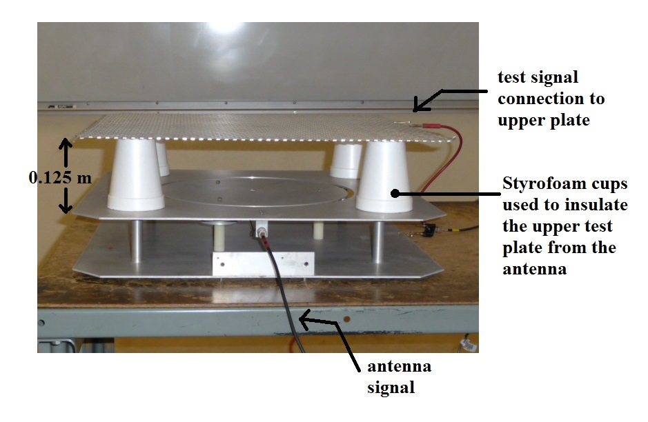
We first need to create a time varying
electric field of known amplitude. We do this by placing
a flat metal screen on insulators a known distance (0.125 m)
above the top of the antenna. A square wave signal from
a function generator is connected to the test plate.
The electric field created by the test screen is just the
voltage on the screen (10 volts) divided by the distance
between screen and the antenna (0.125 m); 80 V/m.
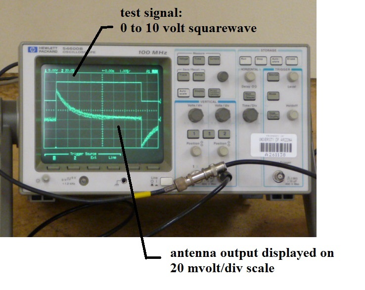
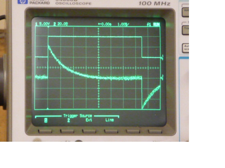
The test signal and the antenna output signal are shown
above. The test signal was a 0 to 10 volt square wave and is
displayed on a 5 volt/div scale above. The antenna signal is
shown below. Note the exponential decay of the signal that
occurs because the 1 M Ω input impedance of the oscilloscope is
connected in parallel with the 1000 pF integrating
capacitor. The signals are being displayed on a 1 ms/div
time scale. A closer view of the oscilloscope display is
shown at right.
We'll do a quick calculation of the voltage that we would
expect from this setup and see how well it agrees with the actual
measurements above.
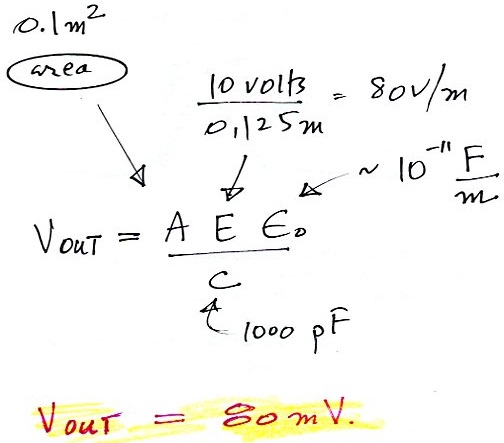
We would expect a peak signal of about 80
mV, we seem to be getting about 60 mV. That's not too
bad. I suspect the reason for the difference is that
there may be some stray capacitance between the antenna and
ground that we would need to add to the 1000 pF in the
integrating capacitor.
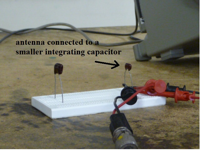
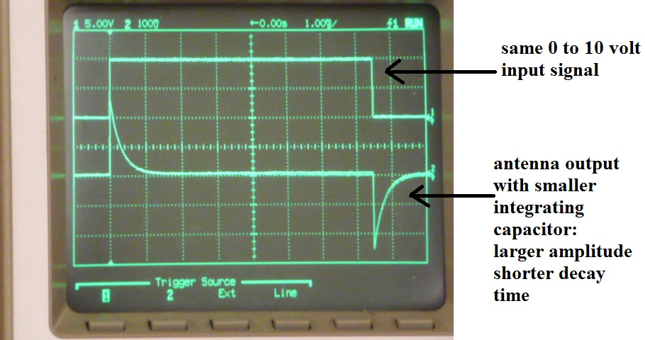
As a final test, the antenna was connected to a small (50 pF)
integrating capacitor. That should increase the
amplitude of the antenna signal and shorten the decay time
constant.
The oscilloscope display above confirms
this. Though again the signal isn't as large and the
time decay as short as calculations would predict. Stray
capacitance is probably again the reason for the
discrepancy. The stray capacitance may well be larger
than the 50 pF integrating capacitor that we are using in this
test.
References:
J.M.
Livingston and E.P. Krider, "Electric Fields Produced by Florida
Thunderstorms," J. Geophys. Res., 83, 385-401, 1978.