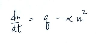
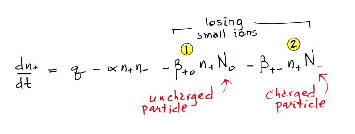
Today we will add two
additional small ion loss terms. A small ion can attach
to an uncharged particle, creating a charged particle or a
so-called "large ion".

Or a small ion of one polarity can attach to a charged particle of the opposite polarity creating an uncharged particle (provided the small ion and the particle have equal quantities of charge). These two new terms are included in the small ion balance equation below. The β+o and β+- terms are referred to as "attachment coefficients."
Or a small ion of one polarity can attach to a charged particle of the opposite polarity creating an uncharged particle (provided the small ion and the particle have equal quantities of charge). These two new terms are included in the small ion balance equation below. The β+o and β+- terms are referred to as "attachment coefficients."
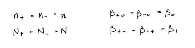
We often assume that the
concentrations of positive and negative small ions and the
concentrations of positively and negatively charged
particles are equal. Let's also make the following
assumptions concerning the attachment coefficients.
The balance equation then becomes
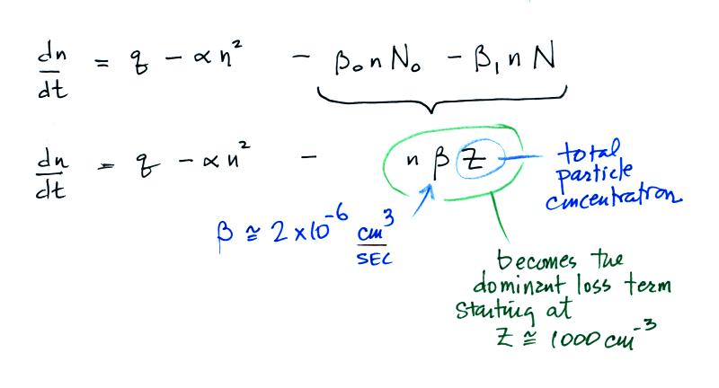
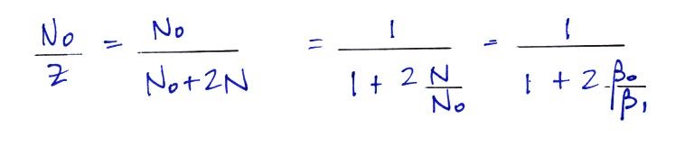
The bottom equation is just an additional
simplification of the top equation. A total particle
concentration term, Z, is used rather than keeping track
of the concentrations of charged and uncharged
particles. This is the form of the equation we'll
use in most situations.
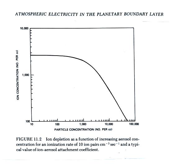
The figure below (from The Earth's Electrical Environment reference) illustrates how ion-particle attachment begins to significantly reduce small ion concentrations beginning at particles concentrations of about 1000 cm-3. Clean air typically has 100s of particles per cc while dirtier air would contain 1000s of particles per cc.
You might remember the research vessel Carnegie mentioned near the start of the semester. In addition to measurements of electric field (the Carnegie curve) measurements of atmospheric conductivity were also made. The instrumentation has changed little since then. Atmospheric conductivity depends on the concentration of small ions which we now see is affected by particle concentrations. There is no question that increased combustion of fossil fuels have increased atmospheric carbon dioxide concentrations; there is concern that this might cause global warming. You might also expect combustion to add particles to the atmosphere. Thus a comparison of atmospheric conductivity made in the early 1900s with measurements made today might provide some indication of whether atmospheric particulate concentrations have changed. Atmospheric conductivity measurements might be another example of proxy data that might be used to track climate change.
We will spend some time considering what fraction of particles are uncharged and charged. We'll start with a large ion (charged particle) balance equation.

Now we'll look at the fraction of large and small particles that are uncharged.
The figure below (from The Earth's Electrical Environment reference) illustrates how ion-particle attachment begins to significantly reduce small ion concentrations beginning at particles concentrations of about 1000 cm-3. Clean air typically has 100s of particles per cc while dirtier air would contain 1000s of particles per cc.
You might remember the research vessel Carnegie mentioned near the start of the semester. In addition to measurements of electric field (the Carnegie curve) measurements of atmospheric conductivity were also made. The instrumentation has changed little since then. Atmospheric conductivity depends on the concentration of small ions which we now see is affected by particle concentrations. There is no question that increased combustion of fossil fuels have increased atmospheric carbon dioxide concentrations; there is concern that this might cause global warming. You might also expect combustion to add particles to the atmosphere. Thus a comparison of atmospheric conductivity made in the early 1900s with measurements made today might provide some indication of whether atmospheric particulate concentrations have changed. Atmospheric conductivity measurements might be another example of proxy data that might be used to track climate change.
We will spend some time considering what fraction of particles are uncharged and charged. We'll start with a large ion (charged particle) balance equation.
N in this equation can
represent the concentration of either positively or
negatively charged particles. Large ions are
created when a small ion attaches to an uncharged
particle. They are destroyed when a small ion
attaches to a charged particle of the opposite
polarity .
Under steady state conditions
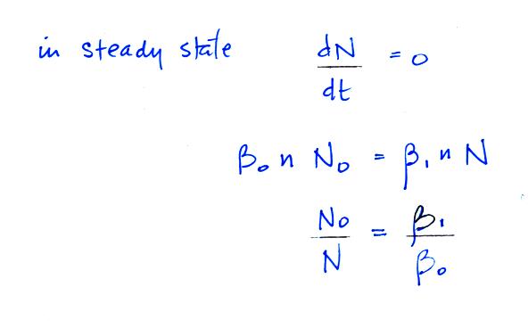
Under steady state conditions
Now we'll look at the fraction of large and small particles that are uncharged.
In some supplementary
notes we look at how a relatively straight
forward solution to the diffusion equation can be used
to derive an expression for β0. You can
then consider the additional flux of small ions to a
charged particle (diffusion plus the effect of the
electric field created by the charged particle).
That gives an expression for β1
. For larger particles we find that
β0
= β1
.
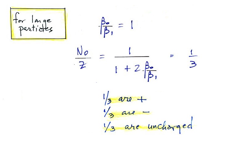
For larger particles you would expect to find equal numbers of positively charged, negatively charged, and non-charged particles.
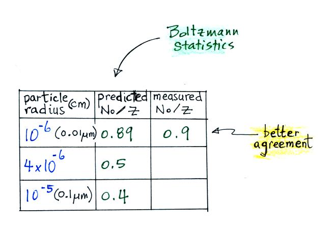
For smaller particles the agreement between predictions and measurements of the uncharged fraction (No/Z) is not very good.
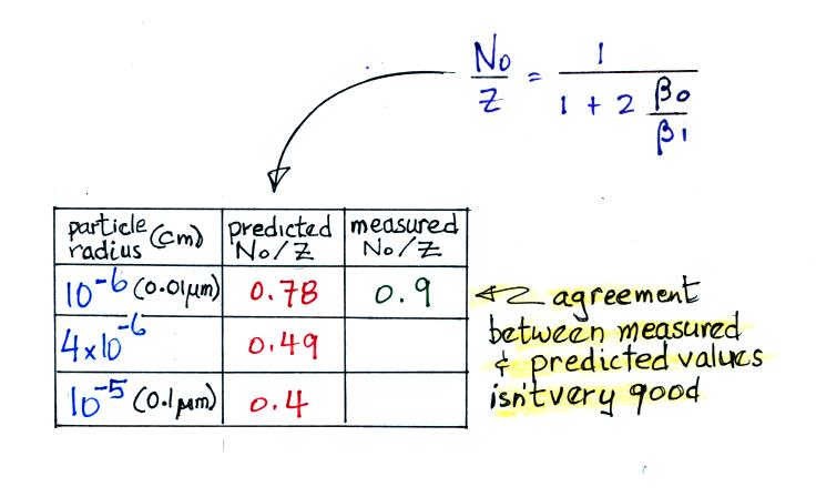
Because of this poor agreement we did not spend any class time working through the details of the diffusion theory approach to estimating particle attachment coefficients. The details are in the supplementary reading though if you are interested.
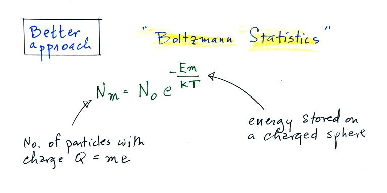
We will have a more careful look at an alternate approach that uses Boltzmann statistics.
For larger particles you would expect to find equal numbers of positively charged, negatively charged, and non-charged particles.
For smaller particles the agreement between predictions and measurements of the uncharged fraction (No/Z) is not very good.
Because of this poor agreement we did not spend any class time working through the details of the diffusion theory approach to estimating particle attachment coefficients. The details are in the supplementary reading though if you are interested.
We will have a more careful look at an alternate approach that uses Boltzmann statistics.
A charged particle
has a certain amount of "stored" energy associated
with it. Thus we can use the Boltzmann
distribution above to predict the distribution of
charged particles (the particles can carry only
integral multiples of an electronic charge, i.e. Q
= me, where m is an integer and e is the charge on
an electron).
The energy stored on a charged sphere is (the details of the derivation are in a second set of supplementary notes)
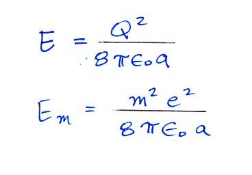
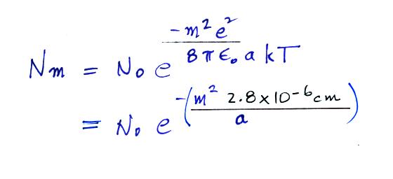
We can insert this expression into the
Boltzmann distribution equation above.
This agrees much better with the measured
value. The table shown earlier is reproduced
below. This time Boltzmann statistics are
used to predict the uncharged fraction.
The energy stored on a charged sphere is (the details of the derivation are in a second set of supplementary notes)
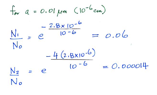
A temperature
of 300 K was assumed in the calculation
above. Also in class I used 0.028 μm in
the parentheses instead of 2.8 x 10 -6
cm. The exponential starts to become pretty
small for particles with radii less that 2.8 x
10-6 cm,
less than 0.028 μm
(especially if m > 1, that is the particle
has more than one electronic charge). So
we can see that most small particles will be
uncharged. Those that are charged will
mostly just carry 1 electronic charge.
For example
Now we can
compare predictions of the uncharged
fraction of particles with
measurements. Here are the details
of the predicted value for a particle with
radius = 10-6
cm.
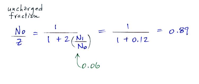
The agreement
between measured and predicted values is much
better. Again, if the table had been
extended to larger particles, we would expect
the predicted No/Z
to approach 0.33.
Next week we will begin to look at thundercloud electrification processes. Here's some supplementary reading that will provide some background information.
Next week we will begin to look at thundercloud electrification processes. Here's some supplementary reading that will provide some background information.