Friday April 10, 2015

Today we will have a brief look at a different way of locating sources of VHF radiation emitted by lightning.  The second part of the class will be devoted to the acoustic signals produced by lightning - thunder.


T
he basic principle involved in interferometry is shown below.


A plane wave of radiation is approaching from the right in the same direction as a line connecting two antennas on the ground.  The antennas are a distance d apart.  Radiation will arrive at Antenna 2 first.  The radiation arriving at Antenna 1 travels an additional distance, l, before reaching the antenna.  The interferometer measures the phase difference, α, in the signals arriving at the two antennas. 

The elevation angle of the arriving signal can then be determined from the measured phase angle,


In order to have a unique solution for the elevation angle, the phase angle can't vary by more than 2π as elevation angle ranges from 0o to 180o


This puts an upper limit on the distance separating the two antennas


In the case where d = λ /2, the phase angle would be π for a signal approaching from the right at θ = 0o (the signal arrives at Antenna 2 before Antenna 1) and phase angle would be -π for a signal arriving from the left at θ = 180o (the signal arrives at Antenna 1 first).   I'm not sure whether a phase detector can distinguish between a phase angle of π and -π or whether it would just measure π in both cases. 

The figure below is a polar plot of the absolute value of the phase angle versus the elevation angle of the incoming signal (for
d = λ /2). 


The circular rings are phase angle varying from 0 at the center of the plot to π at the outer edge of the plot.  There won't be any phase angle difference for signals arriving from overhead (elevation angle, θ = 90o )  because identical features on the signal would reach both antennas at the same time.  This plot leaves the impression that there are two solutions for a single value of the phase angle.  For example, the phase angle is π/2 at Points A and B.  At Point A the signal is arriving at an elevation angle of 60o from the right.  This is shown below.  Point B is a signal arriving at the same elevation angle but from the left.  If the phase detector is able to distinguish between phase angles of +π and -π it would be able to determine whether the radiation was coming from the right or left. 

To illustrate the problem of multiple elevation angles for a given value of phase angle we draw a figure for a larger antenna
separation, d = 2
λ.


Points A, B, C, and D have phase angles of 4π. 2π. -2π and -4π.  These multiple solutions are often referred to as fringes.  At best, the phase detector wouldn't be able to distinguish between 2π and 4π (assuming it would be able to distinguish between positive and negative phase angles) so a measurement of phase angle will lead to at least 2 ambiguous solutions for the elevation angle.  There would be 4 possible elevation angles for a given phase angle measurement if the phase detector is unable to distinguish positive from negative values.  The four labelled points above are shown on a polar plot below.


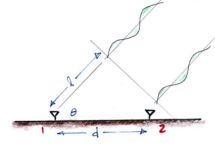
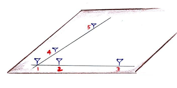
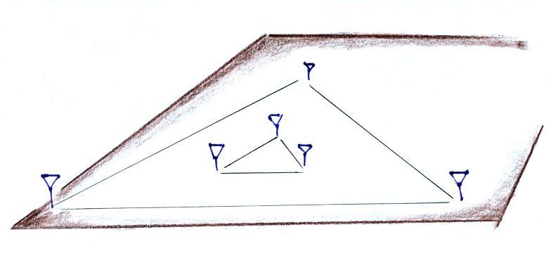
Clearly it would seem like two closely spaced antennas would be best.  However, and we won't go 
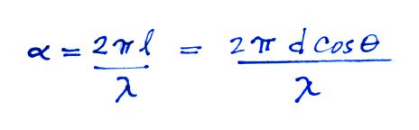
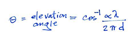
into the details, the error in the elevation angle determination is proportional to 1/d.  So, while there 
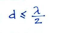
won't be any ambiguities in the elevation angle determination when two antennas are closely spaced, the error could be large.  Two more widely spaced antennas would result in less error but there would be multiple elevation angles possible for a given measured phase angle difference.  What is generally done is to add a 3rd antenna to the baseline as shown below.


A distant antenna to reduce elevation angle error and two close antennas to resolve elevation angle ambiguities.

Up to this point we've been assuming that the direction of the incoming radiation is parallel to the baseline connecting the antennas (i.e. zero azimuth angle).  There is no reason for that to be the case.  As the azimuth angle moves from zero, the measured phase difference will begin to decrease.  The phase angle difference will become zero for a signal approaching from a direction that is perpendicular to the baseline connecting the antennas.  So to be able to determine the true direction angle to the emission source we're going to need a 2nd perpendicular baseline.  Antenna 1 above can be part of both baselines.  So we'll end up with something like shown below. 


An antenna array essentially identical to this was used by Rhodes et. al (1994).  Separation distance between the two inner pairs of antennas was λ/2.  4λ separation was used between the outer pairs of antennas. 


Richard et. al (1986) used 6 antennas arranged in a triangular pattern as shown above.  Spacing between the inner antennas was either
λ/2 or λSpacing between antennas in the outer triangle was 10λ (more than 250 ambiguous elevation angle values).


And finally a brief comparison of lightning source locations from a TOA system (the LDAR network operating at the Kennedy Space Center) and an interferometer developed by the French Office National D'Etudes et de Recherches Aerospatiales (ONERA).  The ONERA system was operated near Orlando, about 60 miles from the Kennedy Space Center in 1992 and 1993.  The results we will be discussing are from Mazur et. al (1997).
 

We mentioned at the beginning of the previous lecture that TOA systems are best able to locate sequences of narrow (pulse widths on the order of microseconds), isolated pulses that are emitted at relatively low repetition rates (1 to 100 pulses per millisecond).   Interferometers are better able to locate the sources of more quasi continuous emissions such as are produced by dart leaders and recoil streamers.


These are time-height plots of VHF radiation sources for an entire storm (adapted from Mazur et. al, 1997).  And actually we're looking at data from two different storms.  The LDAR data is from a storm located over the Kennedy Space Center (over the LDAR network, but far from the ONERA network) that occurred on Aug. 28, 1993.  The ONERA data is from an Aug. 14, 1992 that was close to and in a favorable location for the ONERA network but far from the LDAR system.  Shades of grey give an idea of source density.  The curve on the left side of each figure shows source density as a function of altitude.

Even though we're not looking at observations of the same storm we can draw some conclusions.  The greatest source density for the LDAR data falls between about 6 km and 10 or 11 km which is higher than the ONERA locations where peak density is between the ground and about 7 km.  Radiation sources mapped by the LDAR system remain in the cloud and do not extend to the ground as happens with the ONERA data.

Simultaneous observations of individual discharges by both locating systems were available for only one storm (the Aug. 28, 1993 storm).  An example of an intracloud and a cloud-to-ground discharge are shown below.


Radiation sources are mapped almost continuously during the discharge by the LDAR system.  Source locations also appear in two distinct layers.  This is similar to what Proctor (1991) found when locating the first emissions sources that occur in a discharge.

The sources mapped by the ONERA system appear intermittently with quiet periods in between.  You might be bothered by the fact that the ONERA system shows locations extending down to ground level during an intracloud discharge.  This storm was well outside the nominal range of the ONERA system so the location accuracy is poor.  Both the high source locations (near 20 km) and locations near the ground are due to location errors.  The intracloud discharge did not produce channels that extended down to the ground.


The diamond in this figure indicates the time at which a cloud-to-ground flash was located by the National Lightning Detection Network  There were fewer LDAR locations in this case.  Activity appeared on LDAR throughout the discharge, though locations were mostly confined to the lower of the two layers seen in the intracloud discharge.  Just a few short burst of radiation were located by the ONERA system.  And again, because of the large location errors, we cannot be sure the locations that occur just before 0.2 seconds really did extend down to the ground.

Clearly there are differences in the picture of lightning flashes presented by TOA systems and interferometers.  Mazur et. al (1997) suggests this is "because most of the radiation sources mapped with LDAR are associated with virgin breakdown processes typical of slowly moving negative leaders.  On the other hand, most of the radiation sources maped with ONERA-3D are produced by fast intermittent negative breakdown processes typical of dart leader and K charnges as they traverse the previously ionized channels.  Thus each operational system may emphasize different stages of the lightning flash, but neither appears to map the entire flash."


Thunder

Early in a return stroke, pressure in the channel is several times (maybe a few 10s of times) atmospheric pressure.  The lightning channel expands rapidly outward initially as a shock wave.  Much of the energy in a lightning stroke is dissipated during the formation and outward growth of the shock wave.  The shock wave expands outward a few meters in 10s of microseconds and quickly decays into the sound wave that we eventually hear as thunder.


This figure (this and the next two figures are from an article on Thunder by A.A. Few that appeared in "The Physics of Everyday Phenomena", Readings from Scientific American, W.H. Freeman & Co, San Francisco, 1979) shows the transition from shock wave to sound wave.  The size of the channel when this occurs (a few meters) is referred to as the relaxation radius.  Channel tortuosity features that are smaller than the relaxation radius are swallowed up by the shock wave and don't really affect properties of the thunder such as frequency.


Lightning channels consist first of mesotortuous segments that are 5 to a few 10s of meters long.  Several of these positioned end-to-end and oriented in about the same direction form a macrotortuous segment which is a 100 or a few 100s of meters long.  The variation of sounds that are heard during thunder are determined primarily by your orientation relative to the mesotortuous elements.  Sounds emitted in a direction that perpendicular to the channel are louder than sounds emitted more nearly parallel to the channel.

Microphone A is located more nearly perpendicularly to the 4 mesotortuous segments highlighted in the figure.  Four relatively loud sound pulses arrive in quick succession at microphone A and form a clap of thunder.  Microphone B is positioned more nearly end.  Weaker impulses arrive at the second microphone over a longer period of time and produce more of a rumble.


Another, more realistic, illustration of how the pattern of sounds in thunder and the duration of the thunder depend on your location and the geometry of the lightning channel. 

It is generally not possible to separate the sounds of the separate return strokes in a thunder record (either by ear or on thunder recordings).  A sound that resembles "tearing cloth" has often been reported a split second before the loud clap of thunder from a close lightning strike.  When I mention this in the lecture version of this class, most students agree that they have heard something like this.  The cause of that sound is not known.


At the start of today's notes I mentioned that thunder is one of the loudest sounds in nature.  Because the intensity of sound can vary and is audible over a very wide range it is common to express the intensity of sound in decibel (dB) units.

Intensity = 20 log10 (P/Pref)

Pref  in the equation above is 2 x 10⁻¹⁰ bar (normal atmospheric pressure is approximately 1 bar).

The  chart below (compiled from a variety of sources) lists the intensities of some common sounds.

Intensity
comments
exposure time limit

140
deck of an aircraft carrier

130
jet plane at 100 feet
sound intensity above this level can cause immediate ear damage

120
thunder, chain saw

110
car horn at 1 meter
1 min
100
lawn mower, jack hammer
15 min
95

1 hour
90
sounds above this level regularly cause hearing damage
2 hours
80
garbage disposal, dishwasher, electric shaver, alarm clock

70
radio or TV audio

60
normal conversation

0 dB
threshold of hearing


Thunder duration is examined is a bit more detail in the next figure (from: M.A. Uman, The Lightning Discharge, Ch. 15, Academic Press, Orlando, 1987).


The points on the graph shows actual measurements of thunder duration from discharges at different distances from the observer.  The solid line is a calculation of thunder duration from a vertical lightning channel 7 km tall.  Points A and B highlighted above refer to the calculations below.

Person A in the figure above will hear the thunder coming from the bottom of the channel instantaneously.  Sound travels about 340 m/sec in 20 C air (1 km in 3 seconds, 1 mile in approximately 5 seconds), so the sound from the top of the channel will arrive about 21 seconds later.  That's a duration of 21 seconds.

The observer at Point B will hear the thunder from the bottom of the channel 30 seconds after the lightning strike.  The bottom of the channel is 10 km away from the observer.  The top of the channel is 12.2 km away, so thunder coming from the top of the channel will arrive about 6.6 seconds later than the sound coming from the bottom of the channel
(3 seconds/km x 2.2 km).  The thunder only lasts for about 6.5 seconds at Point B.

Wind can affect the sound of thunder and refraction can mean there is a distance beyond which thunder is not heard


These are pictures of a microphone that has been used to make thunder measurements in the infrasonic to low audio frequency range (a Globe Model 100-B Capacitor Microphone).  The microphone consists of a flexible diaphragm and a metal back plate which act as plates of a capacitor.  The microphone is normally set up right as shown in the left most figure (the metal housing is sometimes covered with a "rubberized hair" wind screen (similar to the "rat's hair" used as a packing material).  The microphone has been turned on its side, in the center picture, to shown the opening that exposes the microphone to the pressure changes caused by thunder.  The right most picture shows the microphone electronics.


Calibrated response of the Globe capacitor microphone.  The microphone response is flat from about 0.5 Hz to about 300 Hz.

Here are three plots of the measured thunder frequency spectra


This first plot is actually a distribution of peak values in sound spectra.  Interestingly a portion of the distribution is below 20 Hz and is inaudible; this is infrasound


This is the spectrum from a single discharge.  The peak in the spectrum is near 100 Hz.


An example of a sound spectrum (lower right corner) that actually peaks in the infrasound. 


Up to this point we have explained thunder as being due to the explosive expansion of a hot lightning channel.  This may not be the cause of all of the emissions at infrasonic frequencies.  Some researchers have suggested that a sudden change in the cloud electrostatic field caused by a lightning discharge might be the cause of the very low frequency infrasonic emissions.


C.O. Hayenga and J.W. Warwick, "Two-Dimensional Interferometric Positions of VHF Lightning Sources," J. Geophys. Res., 86, 7451-7462, 1981.

Mazur, V., E. Williams, R. Boldi, L. Maier, D.E. Proctor, "Initial comparison of lightning mapping with operational Time-Of-Arrival and Interferometric systems," J. Geophys. Res., 102, 11071-11085, 1997.

Rhodes, C.T., X.M. Shao, P.R. Krehbiel, R.J. Thomas, and C.O. Hayenga, "Observations of lightning phenomena using radio interferometry," J. Geophys. Res., 13059-13082, 1994.

Richard, P., A. Delannoy, G. Labaune, and P. Laroche, "Results of Spatial and Temporal Characteristics of the VHF-UHF Radiation of Lightning," J. Geophys. Res., 91, 1248-1260, 1986.