Thursday Sep. 19, 2019
Sia: "California
Dreamin' " (3:37), "Chandelier"
(4:14), "Chandelier"
(4:05), "Midnight
Decisions" (3:44), "Breathe
Me" (4:55), "The
Girl You Lost to Cocaine" (3:58)
We'll be using page
38a, page 38b, page 39a, page 39b, page 39c, page 40a, page 40b, page 40c, page 40d,
(these are mostly pictures, we'll add some
written details in class)
The Troposphere and Stratosphere Optional Assignment has been
graded and was returned today. If you don't see a grade
marked at the top of your paper you earned full credit on the
assignment (0.35 extra credit pts). Here are answers
to the questions on the assignment.
An In-class
Optional Assignment was handed out at the start of class
today and was collected at the end of class. If you weren't
in class and would like to do the assignment you can download the
assignment, answer the questions, and turn in your work at the
start of class next Tuesday.
The Experiment #1 reports are due
next Tuesday. If you haven't returned your materials yet you
can come by my office in Harsbarger 220 today, Friday, or next
Monday. You'll find a box outside my office door where you
can leave the materials. A copy of the Supplementary
Information handout will be nearby. It is important that you
return the materials by next Tuesday at the latest because we need
the glass cylinders for Expt. #2. I am planning on checking
out the Expt. #2 materials next Thursday before the quiz.
The Quiz #1 Study Guide is now
available. Quiz #1 is Thursday next week (Sep. 26).
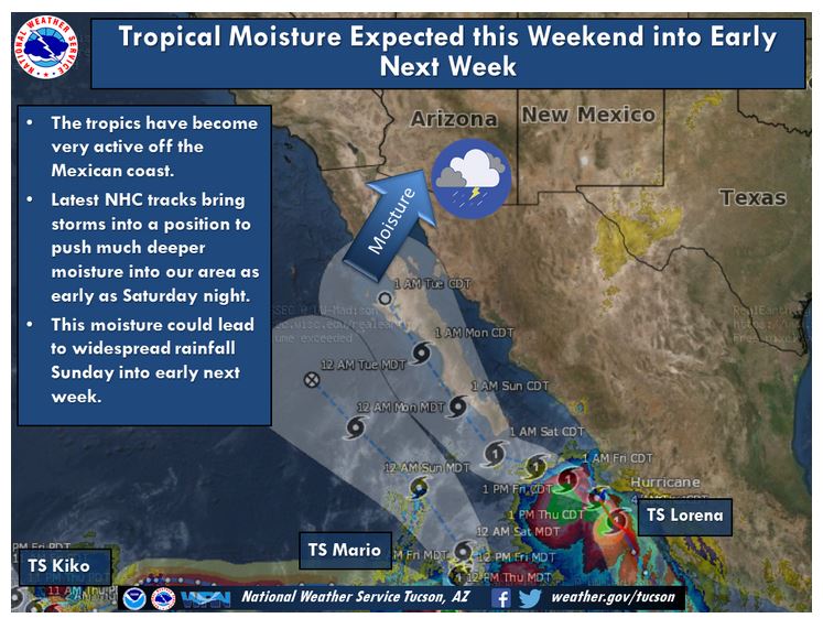
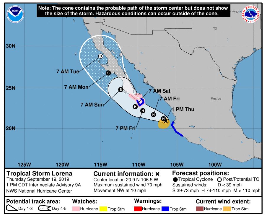
There are a couple of
tropical storms, Lorena and Mario, located off south of Baja
California that may affect our weather this weekend and
early next week.
Both are storms are expected to move north north west in a
track that parallels the west coast of Mexico. (the image
above and the two images below come from the National Hurricane
Center web page
www.nhc.noaa.gov)
|
|
The predicted path of
tropical storm Lorena. Lorena is expected to
intensify to a hurricane (H) then weaken back to tropical
storm strength (S) in the figure above. (D) in the
figure indicates a tropical depression which is a step
below a tropical storm.
|
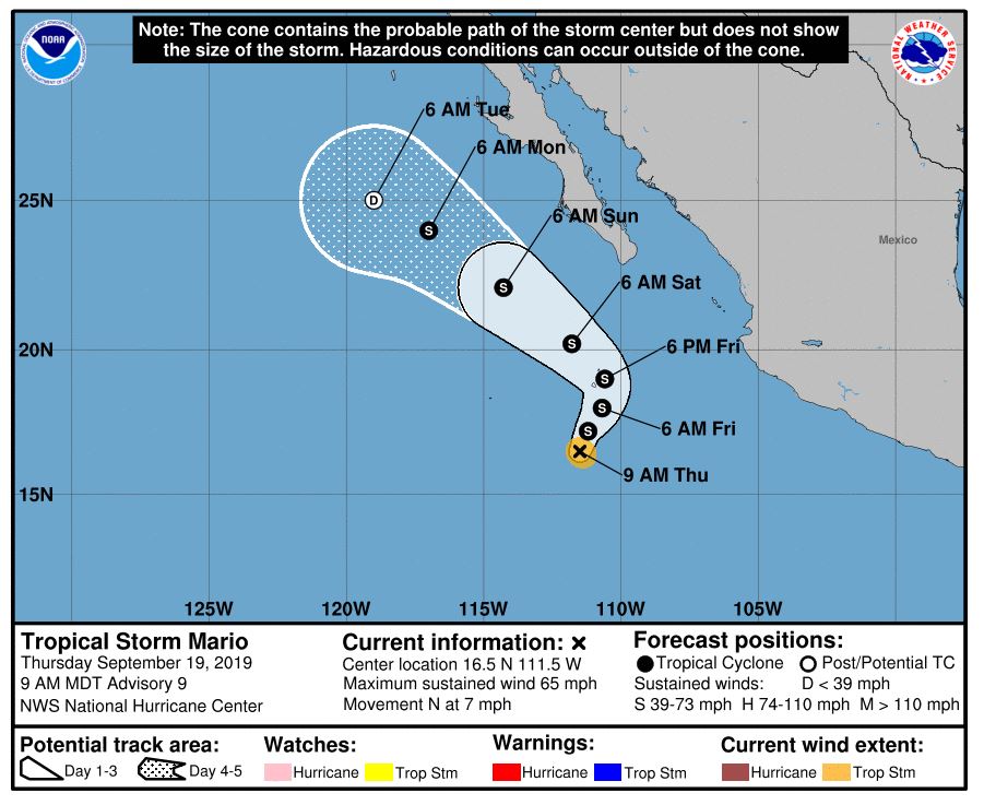
Tropical storm Mario is
expected to follow a similar path though a little further
offshore.
|
We should expect to see an increase in moisture and clouds as
these storms move northward. It is possible that we may also
get some rain early next week.
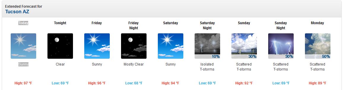
The current weather forecast is
shown below (the images above and below are from the Tucson office
of the National Weather Service
https://www.weather.gov/twc/. The increase in rain chances
for early next week are due to the influx of moisture from Lorena.
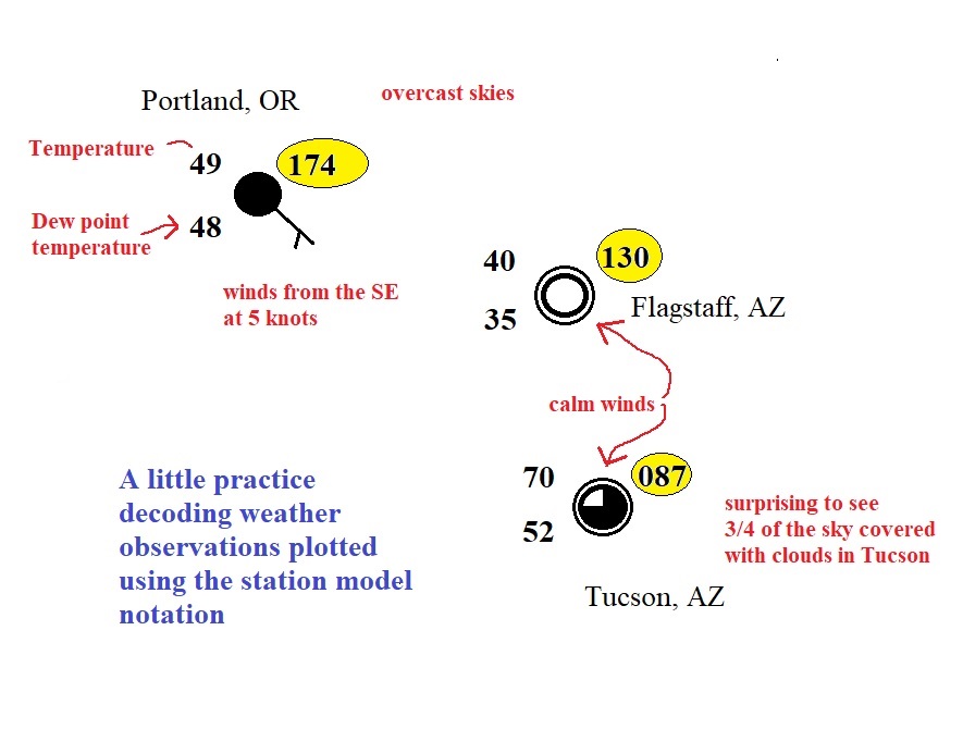
Here are some weather
observations from earlier this morning.
The dew point temperature and the air temperature
(48 F and 49 F, respectively) being observed in Portland were
nearly equal. The relative humidity must have been near
100%.
I was surprised to see such a
difference in the temperatures and the dew point values being
reported in Flagstaff and Tucson. The air in Flagstaff was
quite a bit colder (40 F vs 70 F) and also drier (dew points of 35
F and 52 F) than in Tucson.
We haven't learned what
the numbers highlighted in yellow are. That is pressure
information. That is what we will be starting with today.
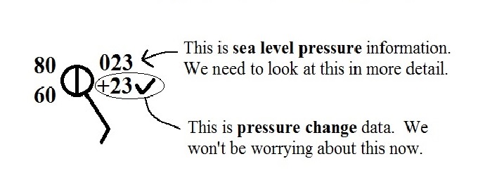
Pressure
The pressure data is usually the most confusing and most difficult
data to decode (page
38a in the ClassNotes)
The sea level pressure is shown above and to the right of the
center circle. Decoding this data is a little "trickier"
because some information is missing. That is done to save
room on the surface map. We'll look at this in more detail
momentarily.
Pressure change data (how the pressure has changed during
the preceding 3 hours) is shown to the right of the center
circle. Don't worry much about this now, but it may come up
next week.
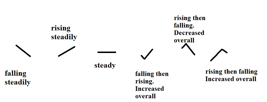
The figures below show the pressure tendency, the symbol following
the pressure change value. This is a visual record of how
pressure has been changing during the past 3 hours.
Again this is something we might use when trying to
locate warm and cold fronts on a surface weather map.
Don't worry too much about it now.
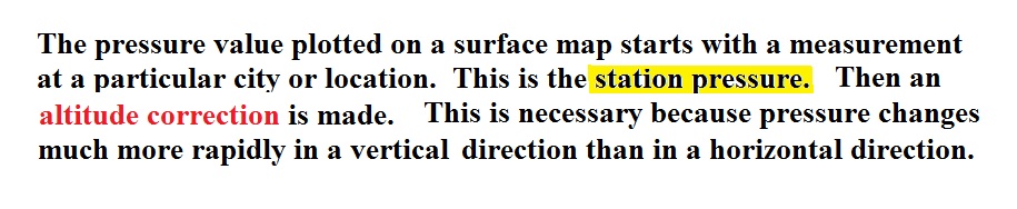
Sea level pressure
Before being plotted on a surface map, pressure data
must be corrected for altitude.
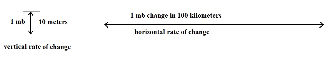
Some typical rates of pressure change are shown below
Meteorologists hope to map out small horizontal pressure
differences on a surface map. It is the small horizontal
differences in pressure that cause the wind to blow and create
storms. If corrections for altitude were not made, the
large vertical changes in pressure caused by altitude would
dominate and would completely hide the horizontal pressure
variations.
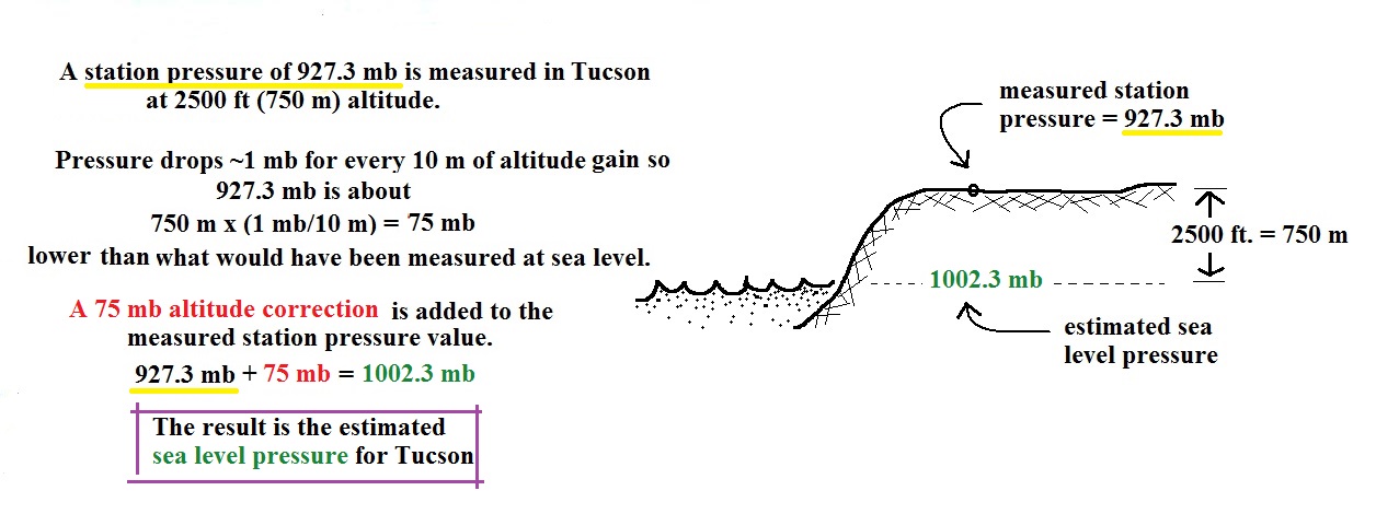
Here's an example of what would be done with a station
pressure measurement made in Tucson.
In the example above, a station
pressure value of 927.3 mb was measured in Tucson. Since
Tucson is about 750 meters above sea level, a 75 mb correction is added
to the station pressure (1 mb for every 10 meters of
altitude). The sea level pressure estimate for Tucson is
927.3 + 75 = 1002.3 mb.
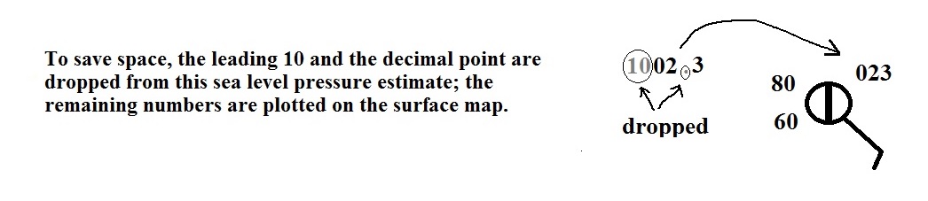
This sea level pressure estimate is the number that gets plotted
on the surface weather map. And actually there is one
additional complication:
To save space only a portion of the full sea level pressure value
is plotted on the map. When reading a weather map you need
to remember to replace the missing 9 or 10 and the decimal point.
Do you need to remember all
the details above and be able to calculate the exact
correction needed? No. You should
remember that a correction for altitude is
needed. And the correction needs to be added to the
station pressure. I.e. the sea-level pressure is
higher than the station pressure.
Coding and decoding pressure
Here are some examples of coding and decoding the pressure
data (page
38b in the ClassNotes)
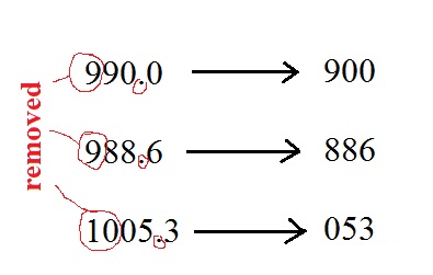
First of all we'll take some sea level
pressure values and show what needs to be done before the
data is plotted on the surface weather
map. Here are more examples than we did in
class.
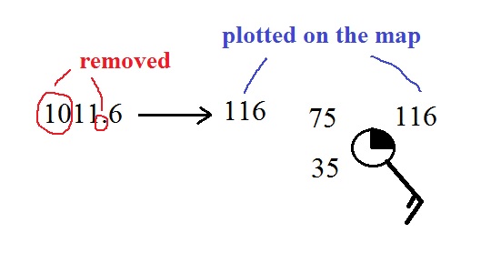
Sea level pressures generally fall between 950 mb and 1050
mb. The values always start with a 9 or a 10. To
save room, the leading 9 or 10 on the sea level pressure value
and the decimal point are removed before plotting the data on
the map. For example the 10 and the decimal
pt in 1011.6 mb would be removed; 116
would be plotted on the weather map (to the upper right of the
center circle). Some additional examples are shown
below.
Here are 3 more examples for you to try (you'll
find the answers at the end of today's notes): 1035.6
mb, 990.1 mb, 1000 mb.
You'll mostly have to go the other direction. I.e.
read the 3 digits of pressure data off a map and figure out
what the sea level pressure actually was. This is
illustrated below.
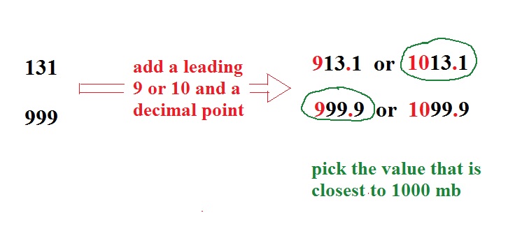
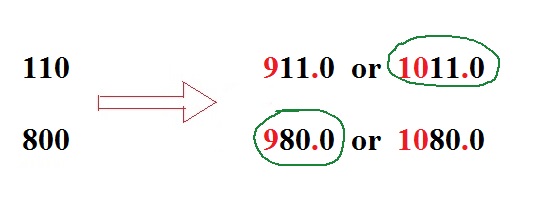
When reading pressure values off a map you must remember to add a
9 or 10 and a decimal point. For example 131
could be either 913.1 or 1013.1 mb. You pick the value that falls closest to 1000
mb average sea level pressure. (so 1013.1 mb would be the correct
value, 913.1 mb would be too low). A couple more
examples are shown below.
Here are a few more examples to try on your own
(answers are at the end of today's notes): 422, 700,
990. Caution: It is values like 990 where you
are likely to make a mistake. The 990 value looks
reasonable, 990 mb. But you do still have to add a leading 9
or 10.
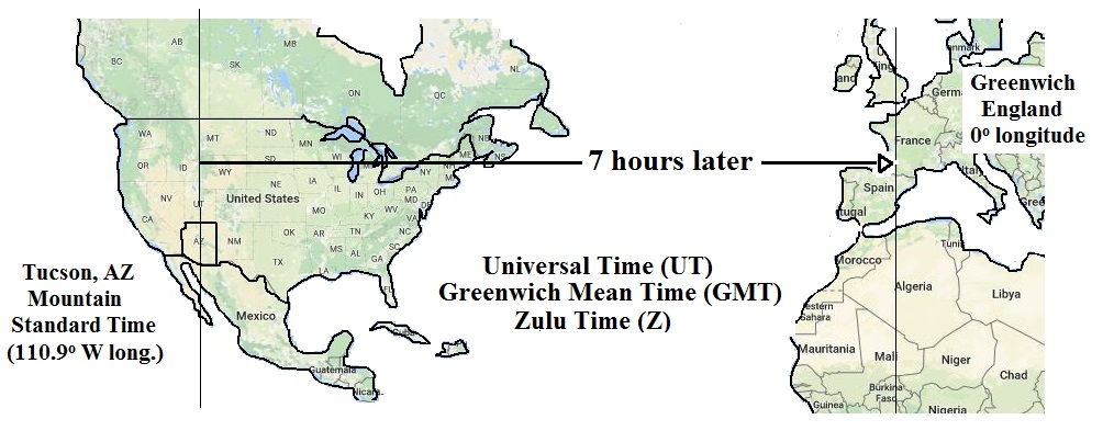
Time
Another important piece of information on a surface
map is the time the observations were collected.
Time on a surface map is converted to a universally agreed
upon time zone called Universal
Time (or Greenwich Mean Time, or Zulu time). That is
the time at 0 degrees longitude, the Prime
Meridian. There is a 7 hour time zone difference between
Tucson and Universal Time (this never changes
because Tucson stays on Mountain Standard Time year round).
You must add 7 hours to the time in Tucson to obtain
Universal Time.
Here are several examples of
conversions between MST and UT (these may differ from the
examples worked in class).
to convert from MST (Mountain Standard Time) to UT
(Universal Time)
10:20 am MST:
add the 7 hour time
zone correction ---> 10:20 + 7:00 = 17:20 UT
(5:20 pm in Greenwich)
2:45 pm MST:
first convert to the 24 hour clock by
adding 12 hours ---> 2:45 pm MST + 12:00 = 14:45 MST
then add the 7 hour time zone
correction ---> 14:45 + 7:00 = 21:45 UT (9:45 pm in
Greenwich)
7:45 pm MST:
convert to the 24 hour clock by
adding 12 hours ---> 7:45 pm MST + 12:00 = 19:45 MST
add the 7 hour time zone
correction ---> 19:45 + 7:00 = 26:45 UT
since this is greater than 24:00
(past midnight) we'll subtract 24 hours ---> 26:45 UT
- 24:00 = 02:45 UT the next day
to convert from UT (Z) to
MST
15Z:
subtract the 7 hour time zone
correction ---> 15:00 - 7:00 = 8:00 am MST
02Z:
if we subtract
the 7 hour time zone correction we will get a negative
number.
So we will first add 24:00 to 02:00 UT --->
02:00 Z + 24:00 = 26:00 Z
next we will subtract the 7 hour time zone
correction ---> 26:00 - 7:00 = 19:00 MST on the previous
day
2 hours past midnight in Greenwich is 7 pm the previous day
in Tucson
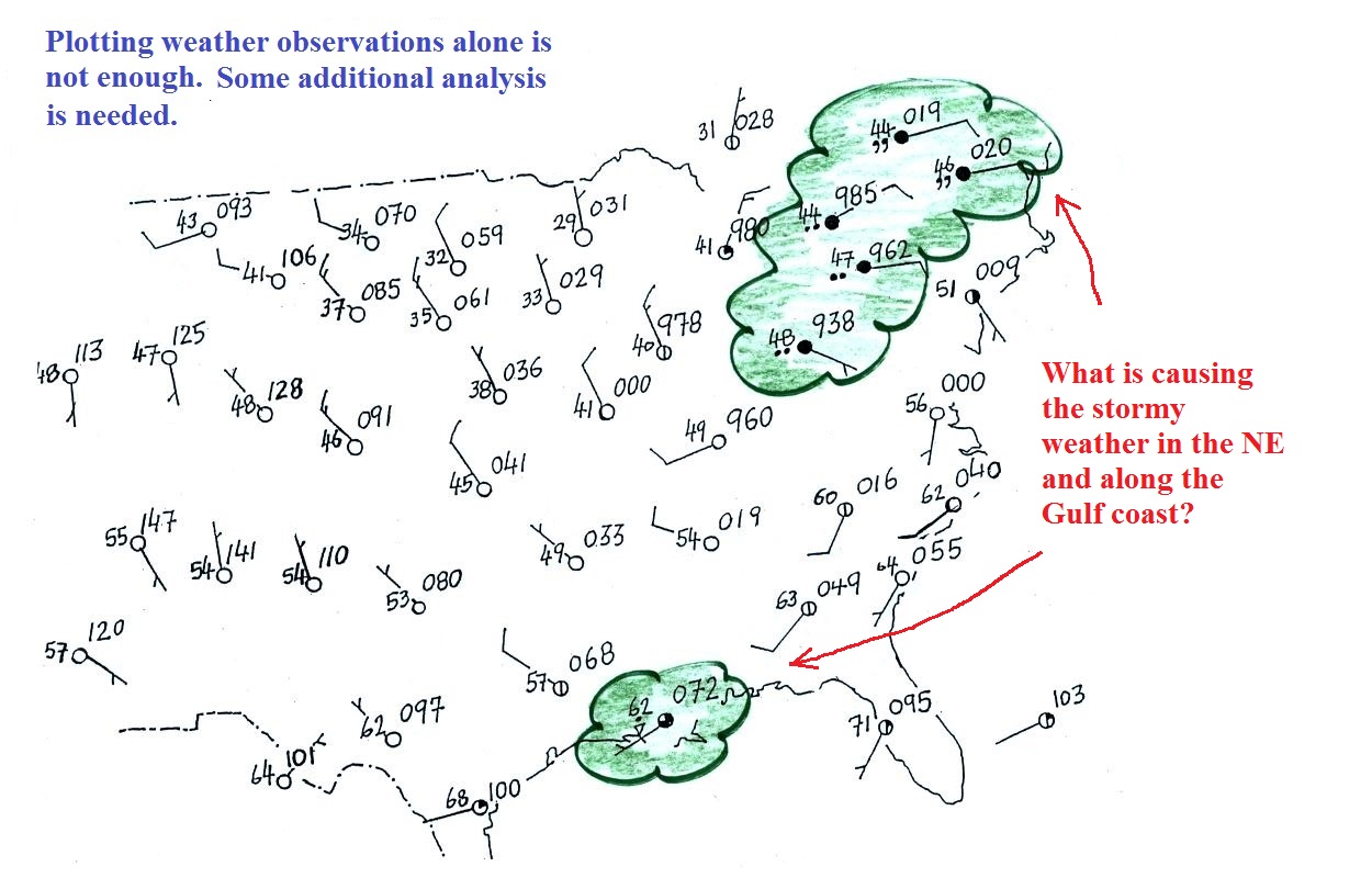
Surface weather map analyses
A bunch of weather data has been plotted (using the
station model notation) on the surface weather map in
the figure below (page
39a in the ClassNotes). A
couple of stormy regions have been circled in green.
Plotting the
surface weather data on a map is just the beginning. For
example you really can't tell what is causing the cloudy
weather with rain (the dot symbols are rain) and drizzle (the
comma symbols) in the NE portion of the map above or the rain
shower along the Gulf Coast. Some additional analysis is
needed.
1st step in surface map
analysis: draw in some contour lines to reveal the large
scale pressure pattern
Pressure
contours = isobars
( note the word bar
is in millibar, barometer, and now isobar ,
they all have something to do with pressure)
Temperature contours = isotherms
A meteorologist would usually begin by
drawing some contour lines of pressure (isobars) to map
out the large scale pressure pattern. We will look
first at contour lines of temperature, they are a little
easier to understand (the plotted data is easier to decode
and temperature varies across the country in a more
predictable way).
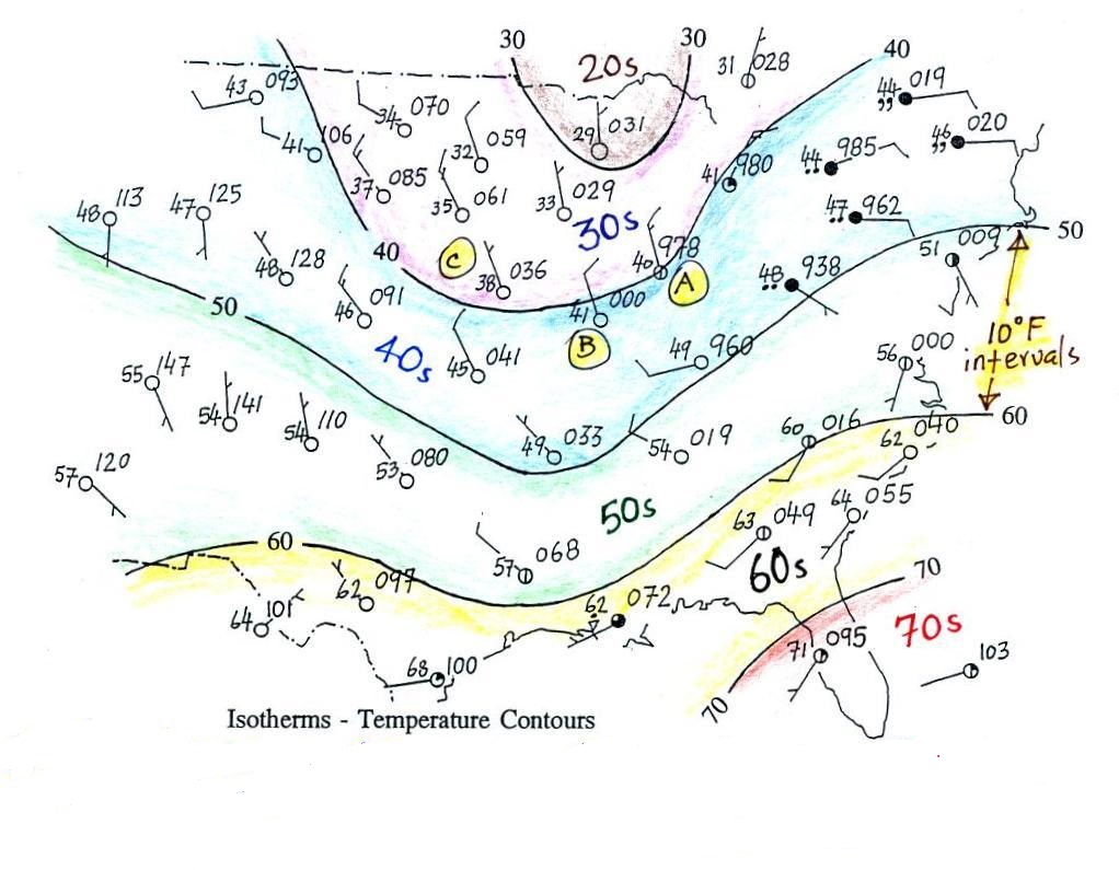
Isotherms
Isotherms, temperature contour
lines, are usually drawn at 10o F intervals. They do two things:
isotherms (1) connect points on the map with the same
temperature
(2)
separate regions warmer
than a particular temperature
from regions colder
than a particular temperature
The 40o F isotherm
above passes through a city which is reporting a temperature of
exactly 40o (Point A).
Mostly it goes between pairs of cities: one with a temperature
warmer than 40o (41o at
Point B) and the other colder than 40o (38o
F at Point C). The temperature pattern is also
somewhat more predictable than the pressure pattern: temperatures
generally decrease with increasing latitude: warmest temperatures
are usually in the south, colder temperatures in the north.
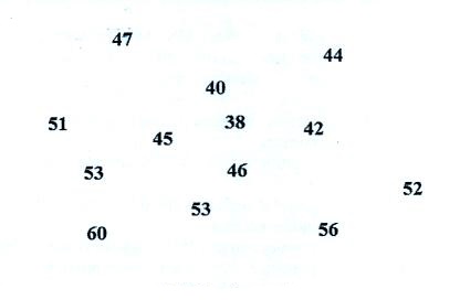
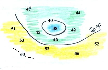
Here's another example starting with just a bunch of temperature
numbers (you'll find this figure on the in-class Optional
Assignment)
Our "job" is to try to make some sense of this data. To
do that we'll draw in 2 or 3 isotherms (40 F, 50 F isotherms and
maybe a small segment of a 60 F isotherm). Colors can help
you do this.
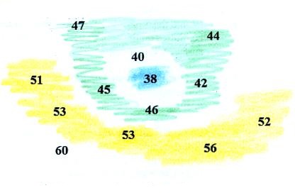
There is one temperature below 40 it has
been colored blue, temperatures
between 40 and 50 are green and temperatures in the
50s are colored yellow. It
should be pretty clear where the isotherms should go.
The isotherms have been drawn in at right; not how the
isotherms separate the colored bands. Note how the 40 F
isotherm goes through the 40 on the map. There is one city
with a temperature of exactly 60 F so a little piece of a 60 F
isotherm is drawn through that city.
Isobars
These are a little harder to draw because you have to
be able to decode the pressure data
isobars (1) connect points on the map with equal pressure
(2) separate regions of high pressure from regions with lower pressure
and
identify and locate centers of high and low pressure
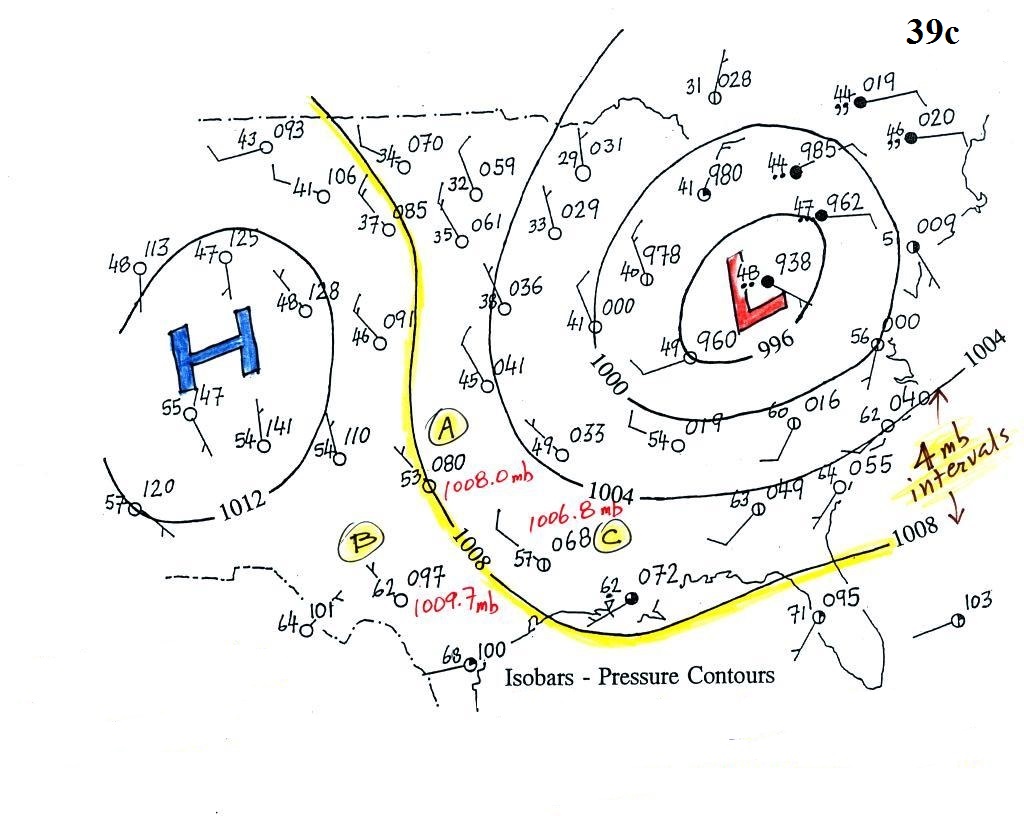
Here's the same weather map with isobars drawn in.
Isobars are generally drawn at 4 mb intervals (above and below a
starting value of 1000 mb).
The 1008 mb isobar (highlighted in yellow) passes through a city
at Point A where the
pressure is exactly 1008.0 mb. Most of the time the isobar
will pass between two cities. The 1008 mb isobar passes
between cities with pressures of 1009.7 mb at Point B and 1006.8 mb at Point C. You would
expect to find 1008 mb somewhere in between those two cites, that
is where the 1008 mb isobar goes.
The isobars separate regions of high and low pressure.
The pressure pattern is not as predictable as the isotherm
map. Low pressure is found on the eastern half of this map
and high pressure in the west. The pattern could just as
easily have been reversed.
This
site (from the American Meteorological Society) first shows
surface weather observations by themselves (plotted using the
station model notation) and then an analysis of the surface data
like what we've just looked at. There are links below each
of the maps that will show you current surface weather data.
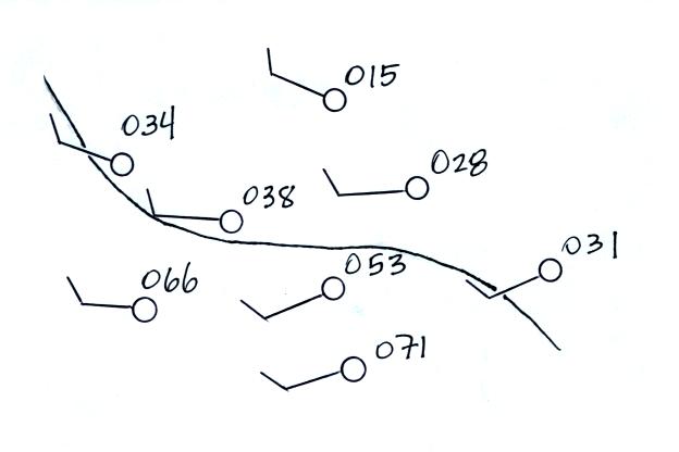
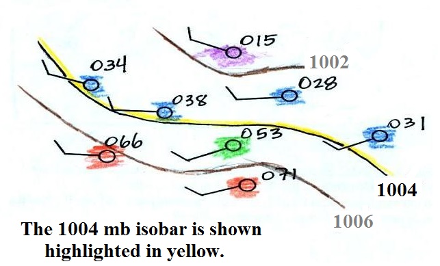
Here's a little practice
A single isobar is shown. Is it the 1000, 1002, 1004, 1006,
or 1008 mb isobar? You'll need to decode the pressure data (add
either a 9 or 10 and a decimal point). You'll find the
answer at the end of today's notes.
What can you begin to learn about the weather once you've draw
isobars on a surface weather map and revealed the pressure
pattern?
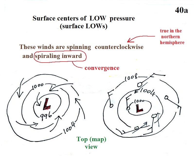
1a. Surface centers of low pressure
We'll start with the large nearly circular centers of High and
Low pressure. Low pressure is drawn below. These
figures are more neatly drawn versions of what we did in class.
Air will start moving toward low
pressure (like a rock sitting on a hillside that starts to roll
downhill), then something called the Coriolis force will cause
the wind to start to spin (don't worry about the Coriolis force
at this point, we'll learn more about it later in the semester).
In the northern hemisphere winds spin in a counterclockwise
(CCW) direction around surface low pressure centers. The
winds also spiral inward toward the center of the low, this is
called convergence. [winds spin clockwise around low
pressure centers in the southern hemisphere but still spiral
inward, we won't worry about the southern hemisphere until later
in the semester]
When the converging air reaches the center of the low it starts to
rise.
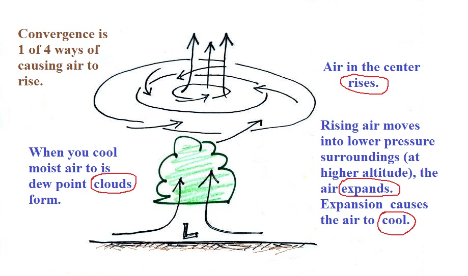
Convergence
causes air to rise (1 of 4 ways)
rising
air e-x-p-a-n-d-s
(it moves into lower pressure surroundings at
higher altitude)
The expansion causes the air to cool
If you cool moist air enough
(to or below its dew point temperature) clouds can form
Convergence
is 1 of 4 ways of causing air to rise (we'll learn
what the rest are soon, and, actually, you already know what
one of them is - warm air rises, that's called convection). You often see
cloudy skies and stormy weather associated with surface low
pressure.
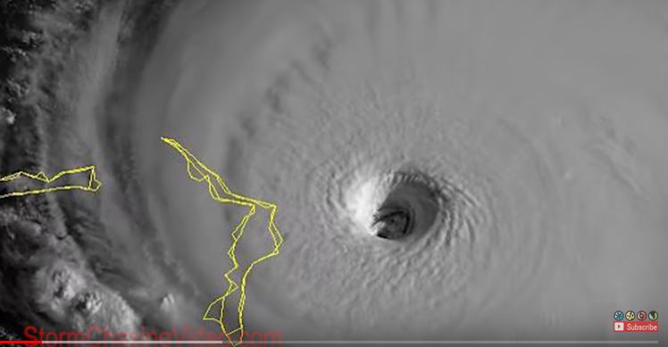
We can see the counterclockwise spinning motions around low
pressure on both radar and satellite observations of Hurricane
Dorian.

|
|
Radar observations of Hurricane as it
approached and then stalled over the Bahamas obtained
from a radar in Nassau. (credit: Brian McNoldy,
Univ. of Miami Rosenthiel School of Marine and
Atmospheric Science, source
of the loop)
|
Visible satellite photography of
Hurricane Dorian on Sep. 1, 2019 (source
of the loop)
|
Converging winds generally produce rising air motions in the
very center of surface low pressure. In the case of a
hurricane the rising air motions are found in a ring of strong
thunderstorms, the eye wall, that surrounds the center of the
storm. Air actually sinks in the center of a
hurricane. This sinking air produces clear skies and
produces the distinctive huricane eye.
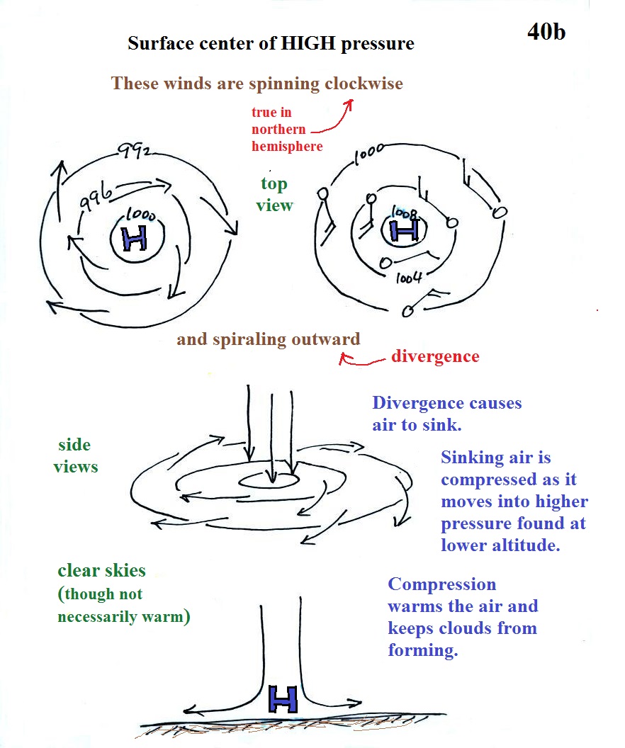
1b. Surface centers of
high pressure
Everything is pretty much the exact
opposite in the case of surface high pressure.
Winds spin clockwise (counterclockwise in the
southern hemisphere) and spiral outward. The outward
motion is called divergence.
Air sinks in the center of surface high pressure to
replace the diverging air. The sinking air is compressed
and warms. This keeps clouds from forming so clear skies
are normally found with high pressure.
Clear skies doesn't necessarily mean warm weather, strong
surface high pressure often forms when the air is very
cold.
Divergence causes air to sink
sinking air is compressed and warms
warming air keeps clouds from forming - clear
skies
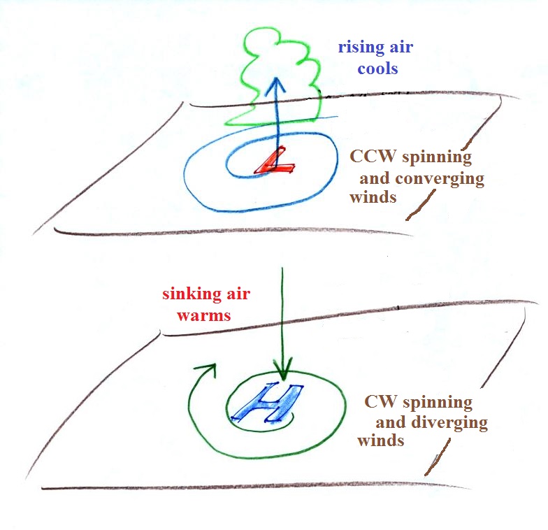
Here's a picture summarizing what we've
learned so far. It's a slightly different view of wind
motions around surface highs and low that tries to combine all
the key features in as simple a sketch as possible.
We were running short on time at this
point. So we will cover what follows at the beginning of
class next Tuesday.
2. Strong and weak
pressure gradients - fast or slow winds
The pressure pattern will also tell you something about
where you might expect to find fast or slow winds. In this
case we look for regions where the isobars are either closely
spaced together or widely spaced. I handed out a
replacement for p. 40c in the ClassNotes (don't throw p. 40c
away).
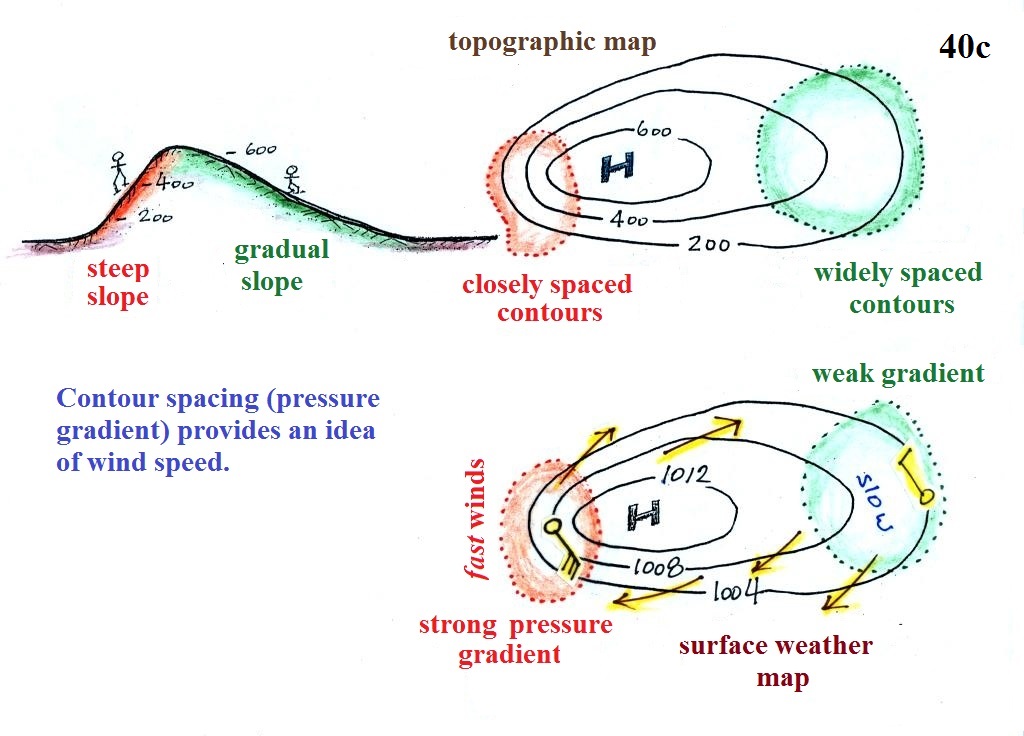
A picture of a hill is shown above at left. The map at
upper right is a topographic map that depicts the hill
(the numbers on the contour lines are altitudes). A center
of high pressure on a weather map, the figure at the
bottom, has the same overall appearance. The numbers on
the contours are different. These are contours (isobars)
of pressure values in millibars.
Closely spaced contours on a topographic map indicate a steep
slope. More widely spaced contours mean the slope is more
gradual. If you roll a rock downhill on a
steep slope it will roll more quickly than if it is on a gradual
slope. A rock will always roll downhill, away from the
summit in this case toward the outer edge of the topographic
map. Air will always start to move toward low pressure
On a weather map, closely spaced contours (isobars) means
pressure is changing rapidly with distance. This is known
as a strong pressure gradient and produces fast winds (a 30 knot
wind blowing from the SE is shown in the orange shaded region
above). Widely spaced isobars indicate a weaker pressure
gradient and the winds would be slower (the 10 knot wind blowing
from the NW in the figure).
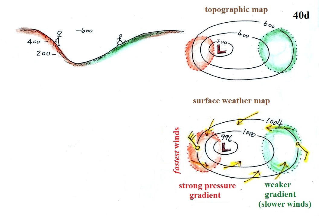
Winds spin counterclockwise and spiral inward around low
pressure centers. The fastest winds are again found where
the contour lines are close together and the pressure gradient
is strongest.
The following figure is on the in-class Optional Assignment.
Contour spacing
closely
spaced isobars = strong pressure gradient
(big change in pressure with distance) - fast
winds
widely spaced isobars = weak
pressure gradient (small change in
pressure with distance) - slow winds
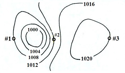
You should be able to sketch in the
direction of the wind at each of the three points and
determine where the fastest and slowest winds would be found.
(you'll find the answer at the end of today's notes).
Once you know which directions the winds are blowing you
should be able to say whether the air at each of the points
would be warmer or colder than normal.
Answers
to the questions about coding and decoding surface weather map
pressure data embedded in today's notes:
Coding pressures (you must remove the leading 9 or 10 and the
decimal point.
1035.6 mb ---> 356
990.1 mb ---> 901
1000 mb = 1000.0 mb
---> 000
Decoding pressures (you must add a 9 or a 10 and a decimal point)
and pick the value closest to 1000 mb.
422 ---> 942.2 mb or 1042.2
mb ---> 1042.2 mb
700 ---> 970.0 mb or 1070.0
mb ---> 970.0 mb
990 ---> 999.0 mb or 1099.0 mb ---> 999.0 mb
Here are a couple more questions embedded in the today's notes.
The isobar in the earlier figure is the 1004 mb contour.
It separates pressures less than 1004 mb (colored blue and violet)
from pressures greater than 1004 (green and orange). The
1002 mb and 1006 mb isobars have also been drawn in (isobars are
normally drawn at 4 mb intervals, so the 1002 mb and 1006 mb
contours wouldn't normally be included).

First the Low and High pressure centers
have been labeled. The brown arrows show the winds
blowing counterclockwise and inward around the Low, clockwise
and outward around the High. Winds are shown using the
station model notation at Points #1, #2, and #3 so that an
idea of wind speed could be included. The isobars are
most tightly spaced (strong pressure gradient) at Point
#3. That's where the fast winds are shown. The
wind at Point #2 is coming from the south, that's where the
warmest air would most likely be found. Colder winds
coming from the NW are found at Points #1 and #3.