Numerical Weather Prediction

Most weather forecasts today are based on the output of complex computer programs, known as forecast models, which typically run on supercomputers and provide predictions on many atmospheric variables such as temperature, pressure, wind, and rainfall. A forecaster examines how the features predicted by the computer will interact to produce the day's weather.

Types of interactions considered in a weather forecast Model

Numerical models of weather (and climate as well) are based on the fundamental mathematical equations which describe the physics and dynamics of the movements and processes taking place in the atmosphere, the ocean, the ice and the land. Some of these processes are shown schematically in the figure above. Global weather forecast models are very complex, deal with huge quantity of data, and require a very large number of calculations. Therefore, these models need fast computers with large memory systems. With the latest technology, a 10-day global weather prediction can be completed in an hour or less.

First, the individual elements that make up the model must be specified along with measurable quantities that define the state of each element. The state of each element, or block, in our model is specified for a given instant of time by a series of numbers that define its temperature, pressure, density, humidity, wind direction and speed, and so on. The diagram below gives you shows you what is meant by individual blocks (or grid cells) within the model.

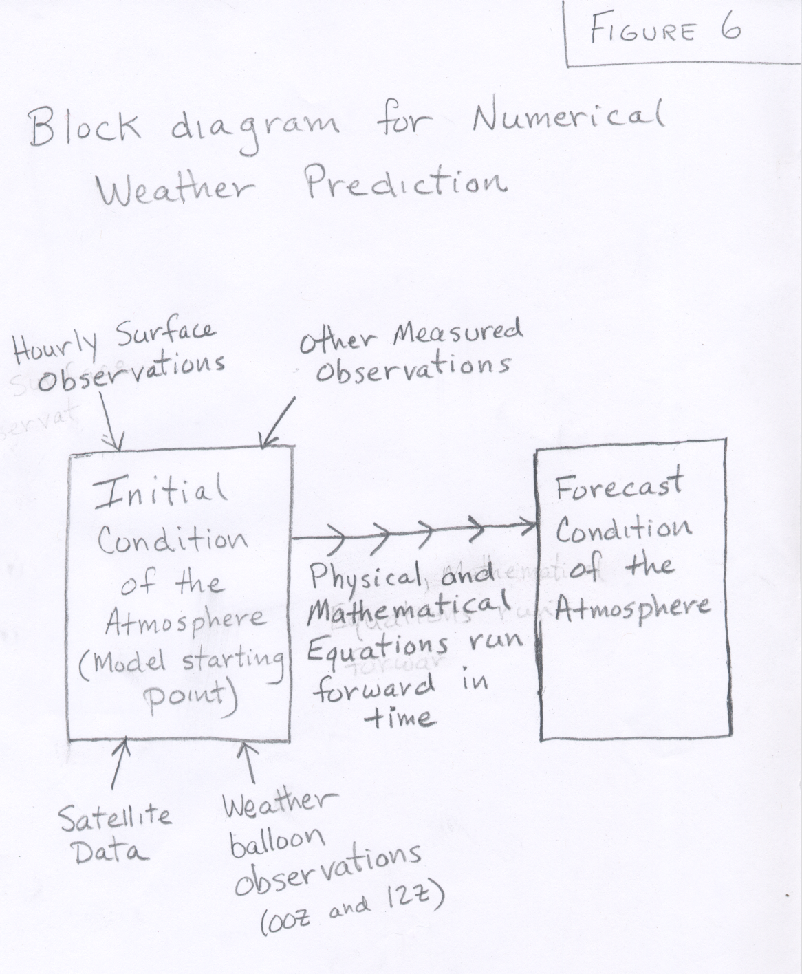
We begin the operation of our model by specifying all these numbers for every block in the model. This is the initial condition of the model and defines the state of the model at the starting time (see Figure 6.)

We can then repeat the process, calculating a new set of changes based on the new state of the model. For global, state-of-the-art weather prediction models, the time step, or time between predicted states of the atmosphere, is about 15 minutes. What we end with is a numerical model that evolves with time, hopefully mirroring changes that will take place in the actual atmosphere. In this class we have looked at forecasts of the 500 mb height pattern. The forecast can be judged by how well the true 500 mb height pattern (at the forecast time) compares with the original forecast.

State of the atmosphere at time t temperature, winds, etc.

equations that describe the behavior of the atmosphere

State of the atmosphere at time t + dt temperature, winds, etc.

equations that describe the behavior of the atmosphere

State of the atmosphere at time t + 2 * dt temperature, winds, etc.

Specifying Initial Conditions

The model forecast must begin with a "known state" of the atmosphere, which is called the initial condition. Most of the information for the initial conditions comes from measurements of the state of the atmosphere. Twice each day, at 00Z and 12Z, weather observing stations launch weather balloons, which carry instruments upward taking measurements of temperature, pressure, winds, humidity, etc. Measurements taken by satellites are also used. The information from around the world is gathered and used to set or initialize the current state of the atmosphere. For example, the measured height of the 500 mb pressure level, taken all over the world, is used to construct the 500 mb height maps we have been looking at.

After gathering all of the observations, the model is run forward in time as discussed above.

Errors in Numerical Forecasts

Unfortunately due to the complexity of the atmosphere, numerical weather forecasts are not exact. There are two main reasons for this. First, the equations used by the models to simulate the atmosphere are not precise. Many processes in the atmosphere are either not fully understood or too complex to model with current computing power. Secondly, the initial conditions are not exact. All measurements have errors. In addition, there are gaps in the initial data since there are many places on Earth where there are no weather observation stations, such as over oceans or unpopulated land areas. Thus, even if the model equations were perfect, if the initial state is not completely known, the computer's prediction of how that initial state will evolve will not be entirely accurate. In fact uncertainty in the intial condition of the atmosphere is what most limits our ability to make accurate weather predictions in the future.

The Earth's atmoshere is a chaotic system, which means that the future state of the system (which is what the model is trying to predict) is highly sensitive to the initial conditions. We know this is true because the same model, run with slightly different initial conditions, will give similar forecasts for the first couple of days, but wildly different forecasts beyond one week into the future (see figure below). In other words, unavoidable errors in specifying the initial conditions tend to amplify with time.

Simple representation of model sensitivity to initial conditions. Suppose we are just looking at the model forecast of temperature for a single location. The three different colors represent forecasts made using the same model, but with slightly different initial conditions. Over the short-term all three model runs make about the same forecast. But at longer forecast times, the three predictions diverge from each other.

Research shows that beyond about 12 days, numerical forecasts models have little skill in predicting weather, that is, you could intellegently guess the weather 12 days from now as well as it can be predicted by current forecast models. Most often, the forecasts are very good in the short term (1-5 days), still decent out to about 6-9 days, but degrade quickly after that.

Dilemma for Weather Forecasters

The public expects precise weather forecasts. As described above, numerical weather forecasts, which are the best we can do, are inherently uncertain. To make matters more confusing, there are dozens of weather forecast models run each day, and each one gives a different forecast. The local weather forecaster will often look over a bunch of models, then add in his knowledge of local weather pecularities, to come up with his individualized forecast. You should expect good short term forecasts and rather poor long range forecasts because that is the best that we can do today. It is not always because the forecaster does not know what he is doing. There is a limit to how well the future state of the atmosphere can be predicted.

Ensemble Weather Forecasting

In an attempt to sort out some of the difficulties in weather forecasting due to uncertain initial conditions, most major operational weather forecasting facilities worldwide now utilize something called ensemble forecasting. In ensemble forecasting each computer weather forecast model is run many times, but with slightly different initial conditions. The sets of initial conditions for each run all fall within the known uncertainty in the worldwide measurements of the initial conditions. Ideally, then the different "members" of the ensemble forecast would each provide a realistic possibility of what might occur in the future ... unfortunately, we cannot say which individual run will turn out to be the most correct. The spread (differences among ensemble members) can be used to make a probability forecast. For example, suppose 20 different emsemble forecasts are made by a particular weather model. Let's say 15 members forecast a strong trough to form over the western United States in nine days, while the other 5 members forecast a ridge to form over the western United States in nine days. While we do not know which of the 20 forecasts will be most correct, we can apply statistics to say, there is a 75% chance (15/20) of a strong trough forming and only a 25% chance (5/20) of a ridge forming in nine days. As of now, these types of probability forecasts are not provided to the public because it is unknown how the public would react and interpret them.

The range of different forecasts from an ensemble prediction can give us an idea about how slight uncertainty in initial conditions lead to forecasts that become highly uncertain the longer out in time the forecast is run. Let's take a look at some current ensemble forecast output provided by US National Center for Environmental Prediction (NCEP) NCEP PSD Map Room. Click on the previous link to open a window to NCEP in another tab and follow these instructions: (1) Choose North America Plots; (2) Select "All Times" under the column "500z spaghetti plots". A series of plots is shown starting from the initial condition, the 1 day (24 hour forecast), the 2 day (48 hour forecast), ..., the 15 day (360 hour) forecast. In these plots, during this time of year, the forecast positions of the 5520 meter (blue) and 5820 meter (red) height contours shown. One line is drawn for each "ensemble member", where the ensemble members are assigned slightly different initial conditions (the 00 hour forecast). NCEP uses 42 ensemble members, thus there are 42 individual blue and red lines that indicate the forecast positions of the 5520 meter and 5820 meter height contours from each ensemble member. There are 21 ensemble members for the latest 00Z forecasts and 21 ensemble members for the latest 12Z forecasts. If the ensemble members are in agreement with each other, the individual red and blue lines will lie on top of each other and when they are not in agreement, the individual lines spread away from each other. Notice that for short range forecasts (up to a few days) that the individual lines are generally tightly packed indicating that the forecast accuracy does not depend much on slight errors in the intial conditions, and we can expect decent forecasts. However, for the longer range forecasts, note that there is a large spread in the blue and red ensemble predictions. The plots now look like a loose pile of spaghetti noodles, which is how the name spaghetti plots originated. The large spread at longer forecast times indicates that the forecast is sensitive to slight (unavoidable) errors in the initial conditions, and at this point it is difficult to say which if any of the ensemble predictions is most accurate. In fact, if done correctly, each ensemble member provides an equally likely outcome. It is important to realize that the "operational" model forecasts that were discussed previously as "the GFS forecast" or the "ECMWF forecast" are just one of the ensemble members, i.e., one of the many lines that make up the spaghetti plots. There is no reason to believe that this "operational" member is any more accurate than any of the other ensemble members. Thus, the spread of the ensemble members is an indication of the uncertainty in the forecast.

Plume Diagrams

This section was recently added. You will not be tested on your ability to understand and use the product described below. I hope you find it interesting.

While the spaghetti plots of 500 mb height clearly indicate the large spread of forecast possibilities that arise due to uncertainty in initial conditions as the forecast period increases, it is difficult to visualize how that that translates to a range of possible temperature and precipitation outcomes for a specific location. A very interesting experimental product from NCEP, called plume plots, shows the ensemble variation of predicted temperature, precipitation, and other weather products for specific cities. A simple description of a few basic functions is provided below. Feel free to experiment with the site if you like. Click on this Link to NCEP Plume Diagrams to open this site in a new tab. First, select a city of interest, using the map toward the bottom of the page. For example, you can click on the star at the location of Tucson. Next, select a parameter to plot just above the graph. "3hrly-TMP" plots the predicted air temperature at the selected city, every 3 hours, out to 87 hours, which is slightly more than 3.5 days. The different colored lines represent different ensemble members. This allows one to visualize the range of ensemble temperature predictions. There are 26 ensemble members, plus the black line, which shows the ensemble mean (or average). These can be considered the range of equally likely outcomes for the selected city. Based on the discussion above, we generally expect the spread to get larger as the forecast length increases. Keep in mind that the forecast period only extends out to about 3 and one-half days. The spread would be expected to get larger if the forecast period were extended to 7, 12, or more days into the future. Another interesting forecast parameter is precipitation amount. Select "3hrly-QPF" to see the quantitative precipitation forecast for each 3 hour period in units of inches of precipitation. Forecasting precipitation amounts is more difficult than temperature forecasts, so the spread for precipitation can be large. "Total-QPF" shows the total accumulated precipitation forecasts for the entire 87 hour forecast.

Another site that shows plume diagrams out to 192 hours (8 days) is EMC's plume page set for Tucson accumulated precipitation plumes. You can change the city and weather parameter.

A Helpful Analogy (hopefully)

Some people are surprised that it is so difficult to predict the weather. They figure that if we spend enough research time and money, we should be able to improve indefinitely, but this is not true. For any chaotic system, there are inherent limitations on the predictability of future states.

Consider the problem of predicting the path of a boulder that we push off the top of a hill. Some of the initial conditions for this problem include the direction in which we push the boulder, the weight of the boulder, the shape of the boulder, how hard we push it, and the precise condition of the hilly terrain (e.g., slope, small rocks in the way, small twigs, clumps of vegetation, etc.). Can we expect to know the initial conditions well enough to capture all the possible ways the path of the boulder can be changed? Probably not. This is in spite of the fact that the equations of motion, which govern the movement of the boulder as it rolls down the hill, are known very well. At first our prediction of the path of the boulder would be very good given that we know which way we pushed it, we know the direction it starts moving. As the boulder rolls down, though, it comes to places where it will hit an obstruction, for example a small rock. If it hits on one side of the obstruction, the boulder makes a left turn, a few millimeters to the other side of the obstruction and the boulder makes a right turn. The future movement of the boulder beyond this obstruction depends critically on whether the boulder took a left turn or a right turn after hitting it. This depends on knowing the initial condition of the hill precisely, which we do not. Slight misrepresentations of the initial conditions cause errors which diverge over time as more of these "obstructions" are encountered. In fact if the hill is very high, our model may have no skill in being able to predict exactly where the boulder will be when it gets to the bottom of the hill. (Think about trying to predict where the puck will fall in the Plinko game on the Price is Right or the where the balls will end up in the Wall game). Predicting the future state of the atmosphere is certainly more complicated than the boulder problem.