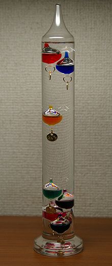
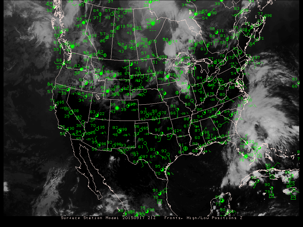
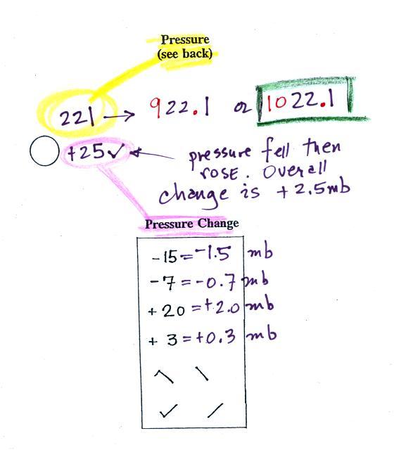
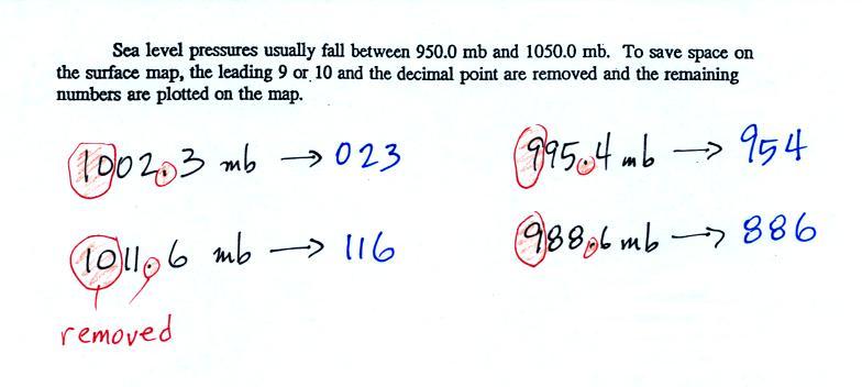
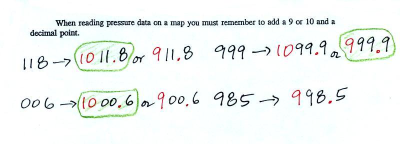
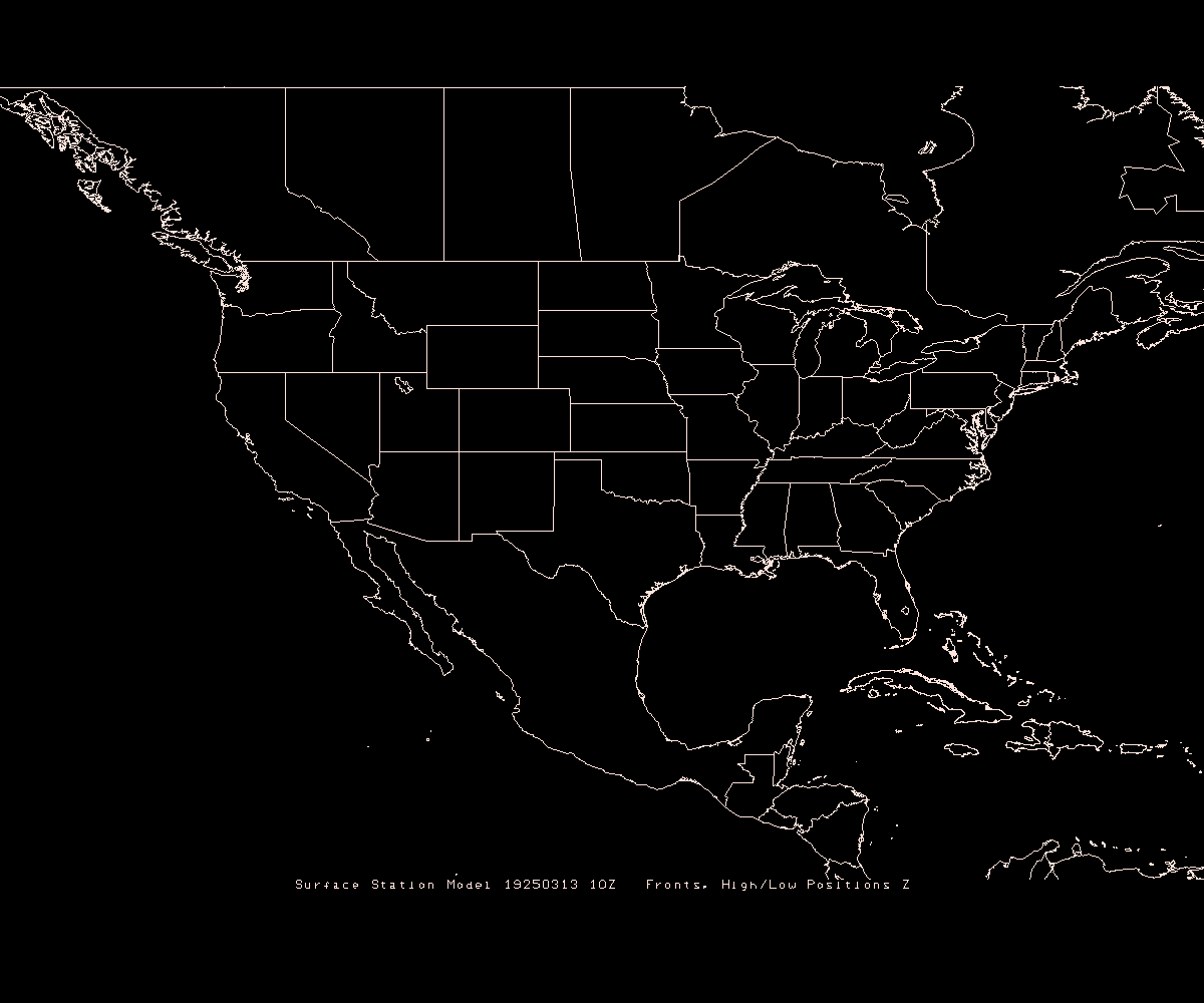
Thursday, Sept. 17, 2015

Music from Adele (live at the Royal Albert Concert Hall): "I'll be Waiting", "If it Hadn't Been for Love", "One and Only"

Quiz #1 is Thursday next week (Sept. 24) and the Quiz #1 Study Guide is now available.  Note that the Tuesday afternoon review will be held from 5- 6 pm in McClelland Park 103.  The Wednesday review will again be from 4 - 5 pm also in McClelland Park 103.

An Optional (Extra Credit) Assignment was handed out in class today.  It was an "in-class" assignment which meant that it was collected at the end of the class period.  If you weren't in class today and would like to do the assignment you can download it and turn it in by the start of class next Tuesday.  You'll receive at least partial credit for the assignment. 

The Experiment #1 reports are due next Tuesday.  You can bring the materials by my office today, Friday, or next Monday and pick up the Supplementary Information handout if you want to.  There'll be a box just inside my office door where you can leave the materials even if it's not during my normal office hours (my office is in PAS 588 and the door should be open between 10 am and 5 pm).

I'm currently planning to distribute the Experiment #2 materials before the quiz next Thursday (Sept. 24).  Expt. #2 uses the same graduated cylinders that were used in Expt. #1 so it is important that they be returned by next Tuesday.

The 1S1P Scattering of Sunlight reports were collected today.  We're currently reading and grading the Carbon Dioxide reports.


Archimedes' principle
Here's another way of trying to understand why warm air rises and cold air sinks - Archimedes Law or Principle (see pps 54a & 54b in the ClassNotes).  It's perhaps a simpler way of understanding the topic.  A bottle of water can help you to visualize the law.


A gallon of water weighs about 8 pounds (lbs).  I wouldn't want to carry that much water on a hike unless I really thought I would really need it.

Here's something that is kind of surprising.


If you submerge the gallon of water in a swimming pool, the jug becomes, for all intents and purposes, weightless.  The weight of the water (the downward gravity force) doesn't just go away.  Once the jug is immersed, an upward force appears and it is strong enough to cancel out gravity.  Archimedes' recognized that this would happen and was able to determine how strong the upward force would be.


In this case the 1 gallon bottle will displace 1 gallon of pool water.  One gallon of pool water weighs 8 pounds.  The upward buoyant force will be 8 pounds, the same as the downward force.  The two forces are equal and opposite.

What Archimedes law doesn't really tell you is what causes the upward buoyant force.  You should know what the force is - it's the upward pressure difference force.


We've poured out the water and filled the 1 gallon jug with air.  Air is much less dense than water; compared to water,  the jug will weigh practically nothing.  But it still displaces a gallon of water and experiences the 8 lb. upward buoyant force.  The bottle of air would rise (actually it shoots up to the top of the pool). The density of the material inside and outside the bottle are the same. A bottle filled with water is weightless. 

Next we'll fill the bottle with something denser than water (I wish I had a gallon of mercury)


Sand is about 50% denser than water.  The weight of a gallon of sand is more than a gallon of water.  The downward force is greater than the upward force and the bottle of sand sinks.


You can sum all of this up by saying anything that is less dense than water will float in water, anything that is more dense than water will sink in water.


Most types of wood will float (ebony and ironwood will sink).  Most rocks sink (pumice is an exception).

The fluid an object is immersed in doesn't have to be water, or a liquid for that matter.  You could immerse an object in air.  So we can apply Archimedes Law to parcels of atmospheric air. 


Air that is less dense (warmer) than the air around it will rise.  Air that is more dense (colder) than the air around it will sink.

Here's a little more information about Archimedes that I didn't mention in class.


There's a colorful demonstration that shows how small differences in density can determine whether an object floats or sinks (we used Coca Cola products in our demonstration; they have the exclusive franchise at the U. of A. at the present time).


A can of regular Coke was placed in a beaker of water.  The can should sink (it did in class).  A can of Diet Coke on the other hand floated.

Both cans are made of aluminum which has a density almost three times higher than water; aluminum by itself would sink.  The drink itself is largely water.  The regular soda also has a lot of high-fructose corn syrup, the diet soda doesn't.  The mixture of water and corn syrup has a density greater than plain water.  There is also a little air (or perhaps carbon dioxide gas) in each can (the diet soda probably wouldn't float if it weren't for the gas in the can.

The average density of the can of regular soda (water & corn syrup + aluminum + air) should end up being slightly greater than the density of water.  The average density of the can of diet soda (water + aluminum + air) is slightly less than the density of water.

In some respects people in swimming pools are like cans of regular and diet soda.  Some people float (they're a little less dense than water), other people sink (slightly more dense than water). 


Many people can fill their lungs with air and make themselves float, or they can empty their lungs and make themselves sink.  People have an average density that is about the same as water.  That makes sense because we are largely made up of water (water makes up about 60% of human males and 55% of human females according to this source)

I wanted to show one last application of some of what we have been learning - a Galileo thermometer.  It's a new acquisition of mine and fairly fragile. 


The left figure above comes from an interesting and informative article in Wikipedia.  The right figure is a closeup view of the thermometer I brought to class.


Here's an explanation of how the thermometers work.  We didn't cover this in class.
This is not something you need to worry about but I included it just in case you're curious.

The fluid in the thermometer will expand slightly if it warms.  It will shrink when it cools. 


The changes in the volume of the fluid will change the fluid's density.  The graph above shows how the fluid density might change depending on temperature.  Note lower densities are found near the top of the graph.


The colored balls in the thermometer all have slightly different densities.  They also have little temperature tags.  The 60 F ball has a density equal to the density of  the fluid at 60 F.  The 64 F ball has a slightly lower density, the density of the fluid when it has warmed to 64 , and so on.  The densities of the floats don't change.


In use the density of the fluid in the thermometer will change depending on the temperature.  The densities of the balls remain constant.  As an example we will that the fluid in the thermometer has a temperature of 74 F.  The 60, 64, 68, and 72 F balls will all have densities higher than the fluid (they lie below the 74F line in the graph above) and will sink.  The remaining balls have densities lower than the fluid and will float.

The lower most floating ball in the illustration has a 76 F temperature tag.  The uppermost of the balls that have sunk reads 72 F.  The temperature is something between 72 F and 76 F.  With this thermometer you can only determine temperature to the nearest 4 F.  Also the thermometer takes quite a while (maybe an hour or two) to respond to a change in temperature.


Surface weather maps
We're starting a new topic today - weather maps and some of what you can learn from them.

We began by learning how weather data are entered onto surface weather maps.

Much of our weather is produced by relatively large (synoptic scale) weather systems - systems that might cover several states or a significant fraction of the continental US.  To be able to identify and characterize these weather systems you must first collect weather data (temperature, pressure, wind direction and speed, dew point, cloud cover, etc) from stations across the country and plot the data on a map.  The large amount of data requires that the information be plotted in a clear and compact way.  The station model notation is what meteorologists use.

Station model notation


A small circle is plotted on the map at the location where the weather measurements were made.  The circle can be filled in to indicate the amount of cloud cover.  Positions are reserved above and below the center circle for special symbols that represent different types of high, middle, and low altitude clouds.  The air temperature and dew point temperature are entered to the upper left and lower left of the circle respectively.  A symbol indicating the current weather (if any) is plotted to the left of the circle in between the temperature and the dew point; you can choose from close to 100 different weather symbols (on a handout distributed in class).  The pressure is plotted to the upper right of the circle and the pressure change (that has occurred in the past 3 hours) is plotted to the right of the circle. 


An example of a surface map like was shown in class today is shown above (this is the 2 pm MST map for Sep. 17 and differs a little bit from the 8 am map shown in class).  Maps like this are available here.  The entry for Tucson has been cut out, enlarged slightly, and pasted in below. 
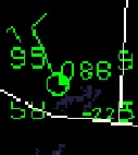
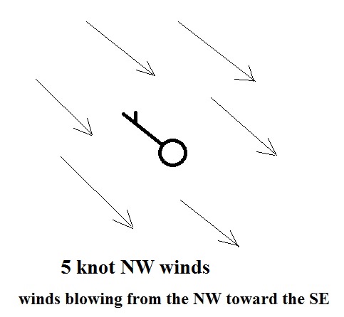
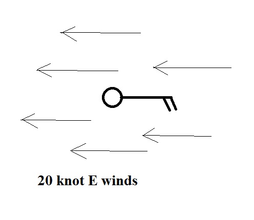
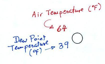


The 2 pm MST weather conditions for Tucson.  The temperature (95 F) and the dew point temperature (58 F) can be 
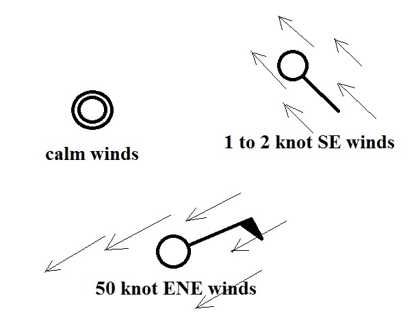
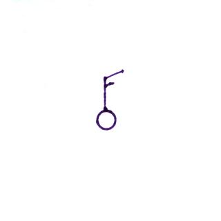
read directly.  Winds were from the NW at 10 knots, this is something you'll learn to decode.  
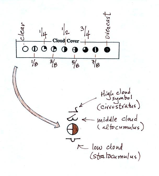
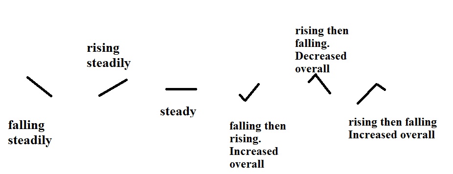
One-quarter of the sky (1/4 of the center circle) was covered with clouds and the (sea level) pressure was 1008.6 mb (derived from the 086 value to the upper right of the center circle).

We worked through this material one step at a time (refer to p. 36 in the photocopied ClassNotes). 
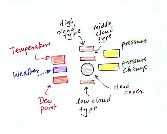
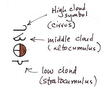
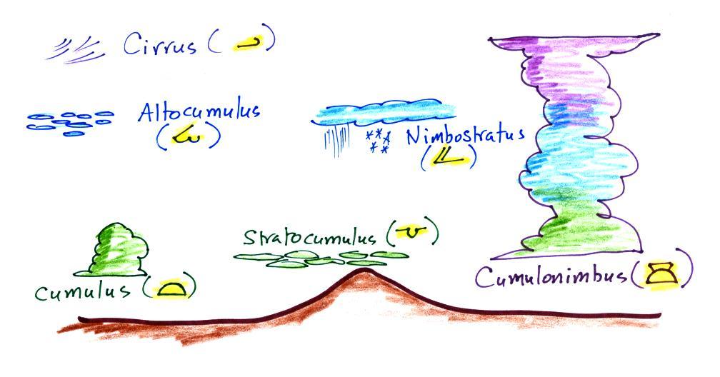
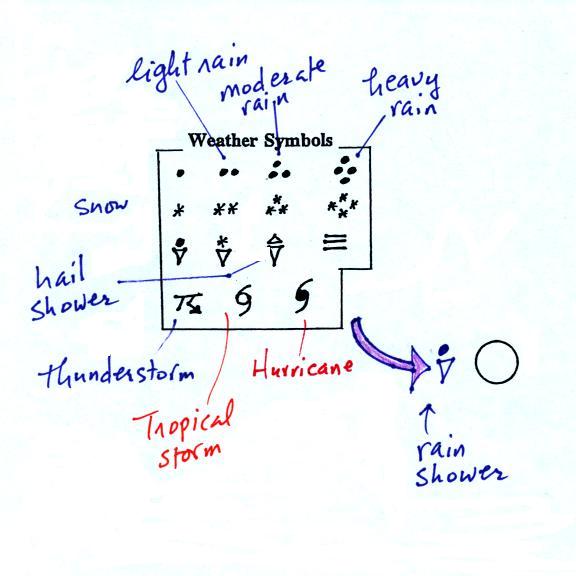
Meteorologists determine how much of the sky is covered with clouds and try to identify the particular types of clouds that are present.


The center circle is filled in to indicate the portion of the sky covered with clouds (estimated to the nearest 1/8th of the sky) using the code at the top of the figure (which I think you can mostly figure out).  5/8ths of the sky is covered with clouds in the example shown.

In addition to the amount of cloud coverage, the actual types of clouds present (if any) can be important.  Cloud types can tell you something about the state of the atmosphere (thunderstorms indicate unstable conditions, for example).  We'll learn to identify and name clouds later in the semester and will just say that clouds are classified according to altitude and appearance.


Positions are reserved above and below the center circle for high, middle, and low altitude cloud symbols.  Six cloud types and their symbols are sketched above.   Purple represents high altitude in this picture.  Clouds found at high altitude are composed entirely of ice crystals.  Low altitude clouds are green in the figure.  They're warmer than freezing and are composed of just water droplets.  The middle altitude clouds in blue are surprising.  They're composed of both ice crystals and water droplets that have been cooled below freezing but haven't frozen.
There are many more cloud symbols than shown here (click here for a more complete list of symbols together with photographs of the different cloud types)

We'll consider winds next.
  Wind direction and wind speed are plotted.


A straight line extending out from the center circle shows the wind direction.  Meteorologists always give the direction the wind is coming from In the example above the winds (the finely drawn arrows) are blowing from the NW toward the SE at a speed of 5 knots.  A meteorologist would call these northwesterly winds. 

Small "barbs" at the end of the straight line give the wind speed in knots.  Each long barb is worth 10 knots, the short barb is 5 knots.  The wind speed in this case is 5 knots.  

Knots are nautical miles per hour.  One nautical mile per hour is 1.15 statute miles per hour.  We won't worry about the distinction in this class, we will just consider one knot to be the same as one mile per hour.   It's fine with me in an example like this if you say the winds are blowing toward the SE as long as you include the word toward.


Winds blowing from the east at 20 knots.


A few more examples of wind directions (provided the wind is blowing) and wind speeds.  Note how calm winds are indicated (the winds were calm in Tucson at class time this morning).  Note also how 50 knot winds are indicated.


Here are four more examples to practice with.  Determine the wind direction and wind speed in each case.  Click here for the answers.

The air temperature and dew point temperature are found to the upper left and lower left of the center circle, respectively.


Dew point gives you an idea of the amount of moisture (water vapor) in the air.  The table below reminds you that dew points range from the mid 20s to the mid 40s during much of the year in Tucson.  Dew points rise into the upper 50s and 60s during the summer thunderstorm season and the dew point was still pretty high this morning.  The summer thunderstorm should be coming to an end in the next week or so and we should notice the drop in humidity when that occurs.  


Dew Point Temperatures (F)

70s
common in many parts of the US in the summer
50s & 60s
summer T-storm season in Arizona (summer monsoon)
20s, 30s, 40s
most of the year in Arizona
10s or below
very dry conditions


And maybe the most interesting part.


A symbol representing the weather that is currently occurring is plotted to the left of the center circle (in between the temperature and the dew point).  Some of the common weather symbols are shown.  There are about 100 different weather symbols that you can choose from.  There's no way I could expect you to remember all of those weather symbols (I certainly don't know many of them myself).

The pressure data is usually the most confusing and most difficult data to decode.


The sea level pressure is shown above and to the right of the center circle.  Decoding this data is a little "trickier" because some information is missing.  We'll look at this in more detail momentarily.

Pressure change data (how the pressure has changed during the preceding 3 hours) is shown to the right of the center circle.  Don't worry much about this now, but it may come up in a week or two.

The figures below show the pressure tendency, they are a record of how pressure has been changing during the past 3 hours.  I didn't show this in class this morning.


Again this is something we might use when trying to locate warm and cold fronts on a surface weather map.  Don't worry too much about it now.

Pressure data
Before being plotted on a surface map, pressure data must be corrected for altitude.


Meteorologists hope to map out small horizontal pressure changes on surface weather maps.  It is these small pressure differences that produce wind and storms. 

Pressure changes much more quickly when moving in a vertical direction than it does when moving horizontally.  There could easily be a 1 mb pressure difference between the floor and ceiling in our classroom.  To see that same 1 mb change when moving horizontally you might need to travel from Tucson to Phoenix,. 

The pressure measurements are all corrected to sea level altitude to remove the effects of altitude.  If this were not done large differences in pressure at different cities at different altitudes would completely hide the important but smaller horizontal changes. 

In the example above, a station pressure value of 927.3 mb was measured in Tucson.  Since Tucson is about 750 meters above sea level, a 75 mb correction is added to the station pressure (1 mb for every 10 meters of altitude).  The sea level pressure estimate for Tucson is 927.3 + 75 = 1002.3 mb.  This sea level pressure estimate is the number that gets plotted on the surface weather map. 

The calculation is illustrated below.


Do you need to remember all the details above and be able to calculate the exact correction needed?  No.  You should remember that a correction for altitude is needed.  And the correction needs to be added to the station pressure.  I.e. the sea-level pressure is higher than the station pressure.

Coding and decoding pressure

To save room, the full 1002.3 mb value from our example above wouldn't be plotted on a surface map.  The leading 10 and the decimal point would be removed.  The 023 that is left over would be plotted on the map as shown in the figure above.

Here are some examples of coding and decoding the pressure data. 


First of all we'll take some sea level pressure values and show what needs to be done before the data is plotted on the surface weather
map.  Here are more examples than  we did in class.

Sea level pressures generally fall between 950 mb and 1050 mb.  The values always start with a 9 or a 10.  To save room, the leading 9 or 10 on the sea level pressure value and the decimal point are removed before plotting the data on the map.  For example the 10 and the decimal pt in 1002.3 mb would be removed; 023 would be plotted on the weather map (to the upper right of the center circle).  Some additional examples are shown above.


Here are 3 more examples for you to try (you'll find the answers at the end of today's notes):

1035.6 mb
990.1 mb
1000 mb

You'll mostly have to go the other direction.  I.e. read the 3 digits of pressure data off a map and figure out what the sea level pressure actually was.  This is illustrated below. 


When reading pressure values off a map you must remember to add a 9 or 10 and a decimal point.  For example
118 could be either 911.8 or 1011.8 mb. You pick the value that falls closest to 1000 mb average sea level pressure. (so 1011.8 mb would be the correct value, 911.8 mb would be too low). 

Here are a few more examples to try (answers are at the end of today's notes)

422
800
990


We didn't have time to cover this remaining information in class today.  We'll probably go over it quickly at the start of class next week.

Another important piece of information on a surface map is the time the observations were collected.
  Time on a surface map is converted to a universally agreed upon time zone called Universal Time (or Greenwich Mean Time, or Zulu time).  That is the time at 0 degrees longitude, the Prime Meridian. There is a 7 hour time zone difference between Tucson and Universal Time
(this never changes because Tucson stays on Mountain Standard Time year round).  You must add 7 hours to the time in Tucson to obtain Universal Time.


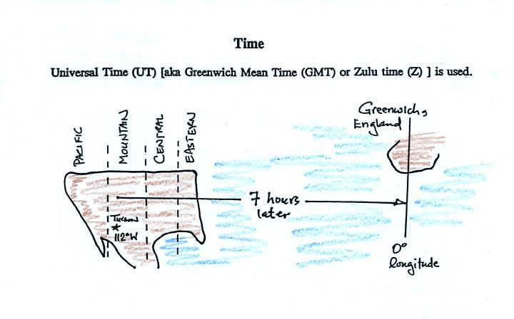
Here are several examples of conversions between MST and UT. 
to convert from MST (Mountain Standard Time) to UT (Universal Time)
10:20 am MST:
add the 7 hour time zone correction --->   10:20 + 7:00 = 17:20 UT (5:20 pm in Greenwich)

2:45 pm MST :
first convert to the 24 hour clock by adding 12 hours   2:45 pm MST + 12:00 = 14:45 MST
then add the 7 hour time zone correction --->  14:45 + 7:00 = 21:45 UT (7:45 pm in England)

7:45 pm MST:
convert to the 24 hour clock by adding 12 hours   7:45 pm MST + 12:00 = 19:45 MST
add the 7 hour time zone correction ---> 19:45 + 7:00 = 26:45 UT
since this is greater than 24:00 (past midnight) we'll subtract 24 hours   26:45 UT - 24:00 = 02:45 am the next day


to convert from UT to MST
15Z:
subtract the 7 hour time zone correction ---> 15:00 - 7:00 = 8:00 am MST 
        
02Z:
if we subtract the 7 hour time zone correction we will get a negative number. 
So we will first add 24:00 to 02:00 UT then subtract 7 hours   02:00 + 24:00 = 26:00
26:00 - 7:00 = 19:00 MST on the previous day
2 hours past midnight in Greenwich is 7 pm the previous day in Tucson


Answers to the questions about coding and decoding surface weather map pressure data embedded in today's notes:
Coding pressures (you must remove the leading 9 or 10 and the decimal point.


1035.6 mb ---> 356
990.1 mb ---> 901
1000 mb = 1000.0 mb ---> 000


Decoding pressures (you must add a 9 or a 10 and a decimal point) and pick the value closest to 1000 mb.

422 ---> 942.2 mb or 1042.2 mb ---> 1042.2 mb
800 ---> 980.0 mb or 1080.0 mb ---> 980.0 mb
990 ---> 999.0 mb or 1099.0 mb ---> 999.0 mb