Friday Jan. 16, 2015


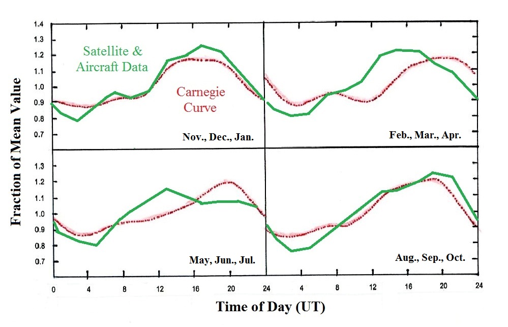
Global electric circuit continued
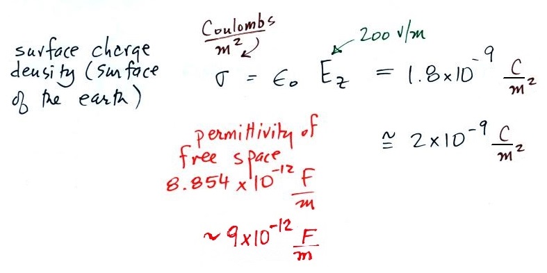
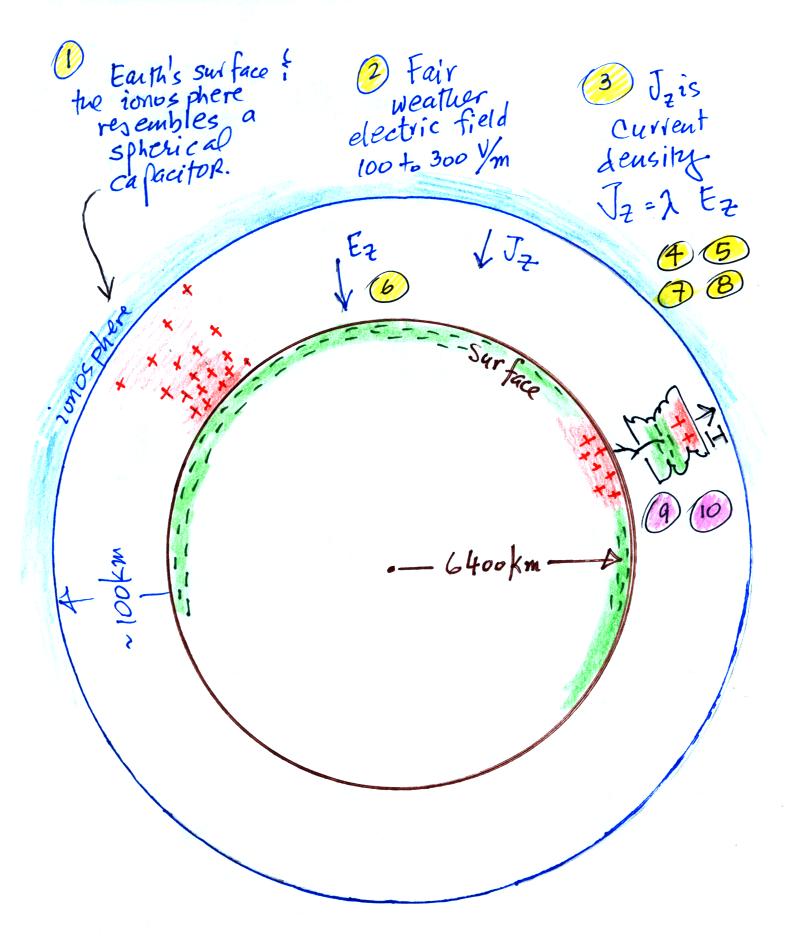
Point 8  There is a simple relation between the surface charge density (Coulombs per unit area) and electric field at the surface of the earth which we assume to be a conductor (we'll derive this expression soon in this class, it's a simple application of Gauss' Law).  F below stands for Farads, units of capacitance.


We'll multiply by the area of the surface of the earth to determine the total charge on the earth's surface


The earth's surface is charged, but a weak current flows through the atmosphere to the earth trying to neutralize the charge on the earth. The following calculation shows that it wouldn't take very long for the current flowing between the ionosphere and the ground, I, to neutralize the charge on the earth's surface, Q.


It would only take about 10 minutes to discharge the earth's surface.  This doesn't happen however.  The obvious question is what maintains the surface-ionosphere potential difference?  What keeps the earth-ionosphere spherical capacitor charged up?


Point 9  The original answer was thunderstorms.  Most cloud-to-ground lightning carries negative charge to the ground which is an upward pointing current.  Corona discharge from objects on the ground (point b) also "sprays" positive charge into the air.  Current also flows upward from the positively charged top of the thunderstorm (the so called "Wilson current" and point c above).

If there are about 2000 thunderstorms active at any time around the globe and each storm sends about 1 A of current upward toward the ionosphere we can account for the 2000 A downward discharging current that we estimated in Wednesday's class. 

At some point it became clear that thunderstorms alone weren't enough.  The thinking then became that electrified shower clouds (ESCs) that are needed together with thunderstorms to produce sufficient charging current.  ESCs are electrified clouds that aren't producing lightning (but they do still contribute to the charging current).

The Carnegie Curve and the global electric circuit charging current
Blakeslee et al. (2014) have recently published results from 15 years of satellite observations of lightning and also electrical measurements made above thunderstorms using high-altitude aircraft.  They address this question of maintaining the earth-ionosphere potential difference and it is worth taking a short detour to look at some of the results of that work. 

We first however need to step back and look at some measurements made in the early 20th century.  The Carnegie, shown below at right, was a research vessel operated by the Carnegie Institution of Washington. 
The Carnegie made seven voyages covering over 300,000 miles between 1909 and 1929 (an explosion in November 1929 killed the captain and burned the ship which was non magnetic and largely built of wood).  The surface electric field was one of many measurements made aboard the Carnegie.  When the surface electric field is measured out over the ocean, where the air is clean, daily variations like sketched below is observed.


A relatively realistic representation of the Carnegie curve adapted from several different sources.
The research vessel Carnegie (image source)

This is known as the "Carnegie curve."  The electric field peaks at around 19:00 GMT (7 pm in London, 12 noon in Tucson) and reaches a minimum at around 04:00 GMT.  It doesn't matter whether the measurements are made in the Atlantic, the Pacific or any other ocean.  The same daily electric field variations are observed simultaneously world wide.  This is because the high conductivity of the two boundaries in the earth-atmosphere spherical capacitor quick spread a local change in voltage difference around the globe.

Air conductivity over the ocean shouldn't very much during the day so a plot of the daily variation of the air earth current density
Jz should have essentially the same shape as the electric field plotted above ( recall the Jz = λ Ez relationship in Wednesday's class).  The Carnegie curve has been described as the "electrical heartbeat of the planet" (I believe that quote comes from R.G. Harrison (2013))

Very early on these variations in electric field were attributed to worldwide thunderstorm activity.  An early comparison is shown below. 


The maximum and minimum values of the world (land) thunder area are about 110 and 40 x 104 km2 .  (adapted from a figure published by F.J.W. Whipple and F.J. Scrase in 1936)


The estimates of thunderstorm activity at the bottom of the figure are based first on the average time of occurrence of thunderstorms at a single location in England.  The same diurnal variation as a function of local time was assumed to apply throughout the world.   Thunderstorm day statistics were also applied to account for different thunderstorm frequencies around the world.  Thunderstorm activity over the ocean was not included.     I should note that I was not able to locate the original reference and am not really sure what the "thunder area" units on the vertical axis represent.

The overall shapes of the Carnegie curve and the plot of worldwide thunderstorm activity are roughly similar. 
But the amplitude variations of the thunderstorm activity are generally larger than the E field variations in the Carnegie curve.  The electric field drops to about 70% of its peak value, the world (land) thunder area drops to about 35% of its peak value. Thunderstorms over land certainly play an important part in keeping the global electric circuit charged up but they are not the whole story. 

This is where the recent data in Blakeslee et al. (2014) come in.  They present data come from 15 years of observations from two satellite sensors in low earth orbit.   Five years of data (1995-2000) come from the Optical Transient Detector (OTD) sensor launched in April 1995.  The OTD detected and located lightning between 75o N and 75o S latitude.  Ten years of data are from the Lightning Imaging Sensor (LIS) launched in November 1997.  The LIS is only able to view lightning at latitudes less than 38o.  Lightning is detected during the day and at night (albeit with different detection efficiencies).  Examples of data from both satellites are shown below (source of the images)


One year's worth of lightning data collected with the OTD
Lightning detected by the LIS from the start of its mission through February 2012

The figure below (a portion of Fig. 3 in the Blakeslee et al. paper) shows the average diurnal variation in lightning flash rate from the OTD/LIS data set.  We'll look at the OTD and LIS sensors as well as the Geostationary Lightning Mapper (GLM) instrument planned for the GOES-R satellite later in the course.


Note that activity over the ocean is included in this figure.  Ocean lightning flash rate remains fairly constant throughout the day.  Activity over land generally peaks between 15:00 and 17:00 Local Time (the minimum occurs between 09:00 and 11:00 LT). 

One of the interesting results that came from these satellite observations of lightning is that the average lightning flashing rate, long thought to be about 100 flashes/second, is actually about half that, 45.7 flashes/second.

Average annual and seasonal flashing rates are shown in the table below (the peak seasonal rate is highlighted for each region in red)

Annual and Seasonal Lightning Flash Rates (flashes/second)
Region
Annual
(Dec., Jan., Feb)
(Mar., Apr. May)
(Jun., Jul., Aug.)
(Sep., Oct., Nov.)
World
45.7
35.9
44.1
55.7
47.2
Land
40.3
31.2
37.7
49.9
42.2
Africa
13.7
12.9
13.9
13.0
15.0
South America
8.8
10.1
6.3
5.6
13.1
Asia
6.5
0.8
8.4
12.4
4.2
Ocean
5.4
4.7
6.3
5.8
4.8
North America
5.4
0.6
4.1
12.9
3.9
Australia
4.4
6.5
3.8
2.2
5.1
Europe
1.6
0.2
1.2
3.9
1.1

Over land the peak flashing rate occurs during the summer, though when examined on a region by region basis, there is not always the case.  Peak flashing rate over South America, for example, occurs during the southern hemisphere spring.  That is probably because convective activity often precedes the beginning of the summer rainy season in the tropics.  Summer flash rates in the northern hemisphere are greater than in the southern hemisphere (more land in the northern hemisphere). 

Averaged over the globe, flash rates over the oceans remain relatively constant throughout the year. 

Blakeslee et al. (2014) also report on 1063 overflights of electrified clouds (thunderstorms and ESCs) collected between 1993 and 2010.  Three different aircraft were used (2 of which were remoted piloted).  Two of the three aircraft made simultaneous measurements of electric fields and conductivity (which then allows estimates of current to be made).  Measurements were made at a surprising number of locations around the world.

The figure below summarizes the measurements of current above thunderstorms and ESCs over land and the ocean.


Over land 77% of the clouds in the study were thunderstorms.  The remaining 23% were ESCs.   There are more electrified clouds over the ocean that are not producing lightning (66%) than there are that are producing lightning (34%).  Over land the average upward current per thunderstorm was 1.0 A (0.13 A for ESCs).  The average current per thunderstorm over the ocean was 1.7 A (0.41 A for ESCs).  The uppermost current values (in kiloamperes) show the average annual current from electrified clouds over the land and ocean.  The overall total average is 2.09 kA.

Thunderstorms over land account for about 52% of the total annual average global circuit charging current (1.09 kA out of 2.09 kA).  Ocean thunderstorms supply 31% of the total.  Electrified clouds over the ocean make a smaller, about 15%, but important contribution.  ESCs over land account for only 2% of the charging current.

We can combine average flash rate determination from satellite observations and measurements of the average flash rate per storm made with the high-altitude aircraft overflights to determine the number of storms active at a particular time [(flashes/second) / (flashes/sec per storm) = no. of storms).  An example is shown in the figure below.


This is for just the three months of June, July, and August (an annual average was not included in Blakeslee et al.).  The number of oceanic storms always hovers around 1000 in all the seasons.  The number of storms over land is more variable but is usually 1000 or somewhat above.  Thus there are always around 2000 storms active at any time around the globe.

Now finally we can combine the data on the number of storms active at a particular time with the average values for currents flowing from individual storms to come up with an estimate of the total global electric circuit charging current.  This estimate is then compared to the Carnegie Curve in the next figure.

The agreement in the Nov., Dec., Jan. and the Aug., Sep., Oct. groups is quite remarkable.  There are some slight phase differences in the other two groups but the overall amplitude variations are very similar. 

Points 1-8 in the figure at the beginning of Wednesday's class (reproduced below) constitute what might be called "fair weather atmospheric electricity."  We'll spend the first 1/3rd,

maybe 40%, of the class working in this area. 


Point 10  Most of the remainder of the class will be devoted to stormy weather electricity, i.e. thunderstorms, lightning, and related topics. 


We'll look at how thunderstorms become electrified (doesn't it seem surprising that electrical charge is created and separated in the cold wet windy interiors of thunderstorms?). 

We'll spend quite a bit of time looking at the sequence of events that make up negative cloud-to-ground lightning.  We'll also look at other types of lightning (intracloud lightning, positive cloud-to-ground lightning, upward and triggered lightning).

We'll look at how lightning current characteristics can be measured either directly or using remote measurements of electromagnetic fields.  This is important because some knowledge of lightning currents characteristics is needed to to design effective lightning protection equipment. 

Lightning causes a lot of damage to electrical transmission and distribution systems and kills just under 100 people per year in the United States.  So we'll learn some of the methods of protecting structures and electrical systems from lightning and how to protect yourself from lightning. 

We'll also look at new ground- and satellite-based sensors being used to detect lightning as it occurs around the globe.

Finally there is usually time enough at the end of the semester to cover a variety of miscellaneous topics such as: volcanic lightning and lightning on other planets, high altitude luminous phenomena associated with lightning (sprites, blue jets, and elves), and the production of x-ray and gamma ray radiation by lightning.


R.J. Blakeslee, D.M. Mach, M.G. Bateman, J.C. Bailey, "Seasonal variations in the lightning diurnal cycle and implications for the global electric circuit," Atmos. Res., 135-136, 228-243, 2014.

R. Giles Harrison, "The Carnegie Curve", Surv. Geophys., 34, 209-232, 2013.