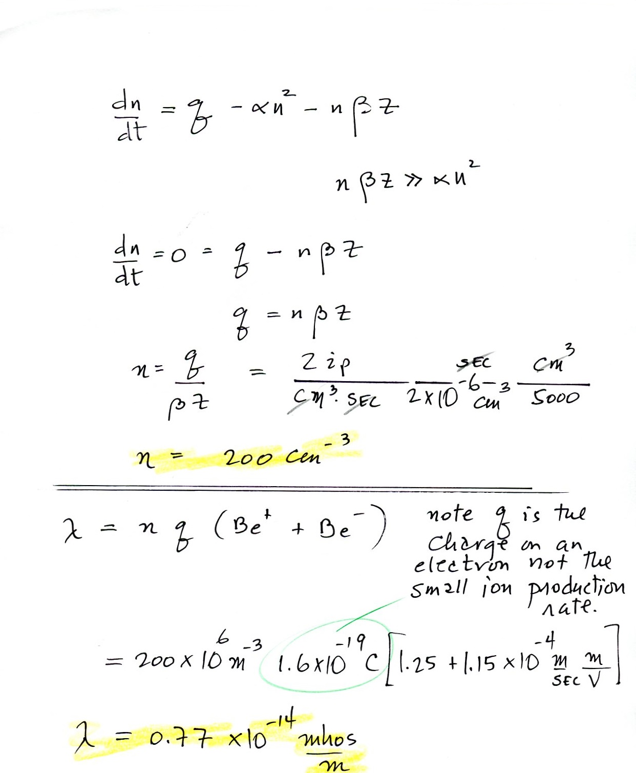
Note the final conductivity value is
somewhat less that what we are used to (we used a value of 2 x
10-14 mhos/m on the first day of
class). This is presumably due to the high particle
concentration and high particle attachment loss rate.
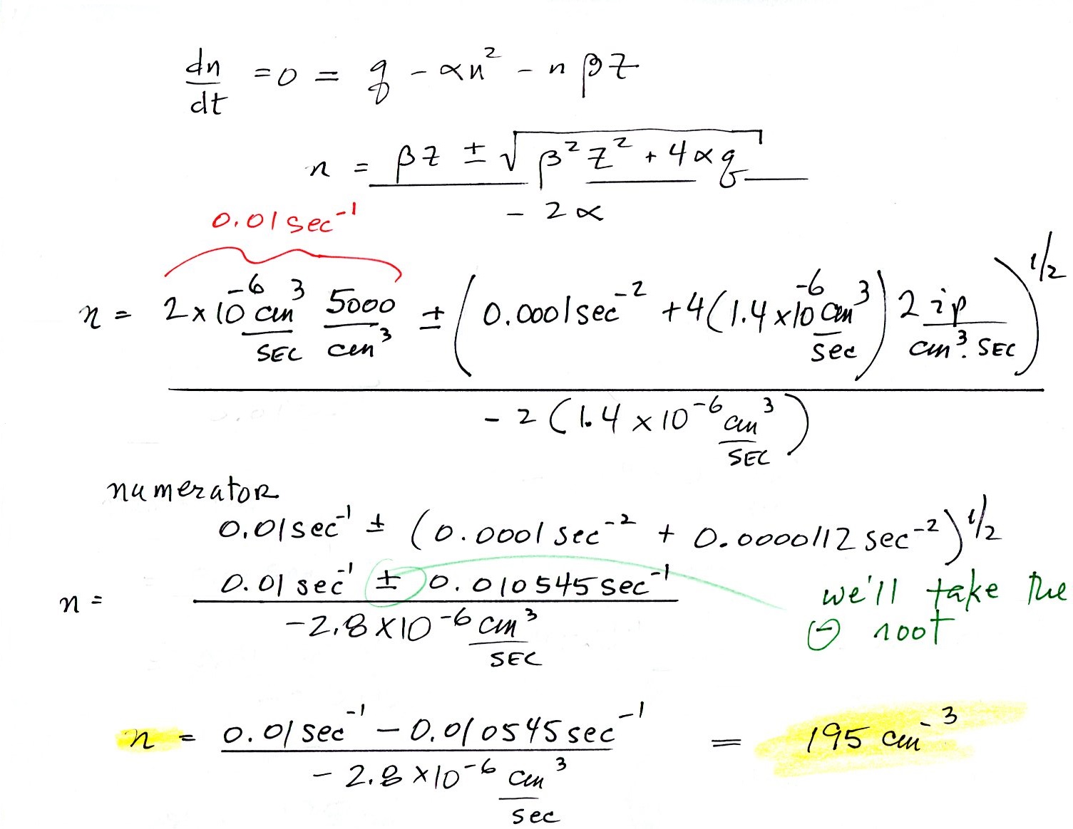
The other half of the class left the recomination term in the small ion balance equation and solved the resulting quadratic equation (the quadratic equation was solved in the notes from the review for the 2013 Midterm Exam). The details of that somewhat more time consuming calculations are shown below.
The other half of the class left the recomination term in the small ion balance equation and solved the resulting quadratic equation (the quadratic equation was solved in the notes from the review for the 2013 Midterm Exam). The details of that somewhat more time consuming calculations are shown below.
Note the final result is very nearly
the same as we obtained when neglecting the recombination
loss term.
3. Most students didn't attempt this question, but it's not too bad.
3. Most students didn't attempt this question, but it's not too bad.
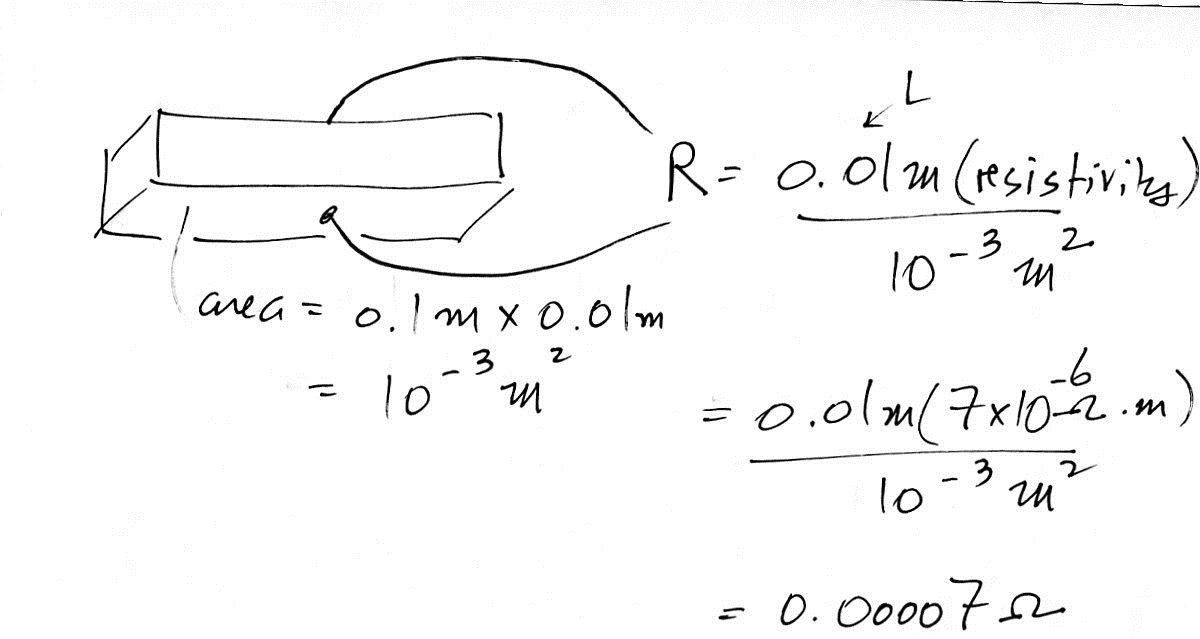
4.
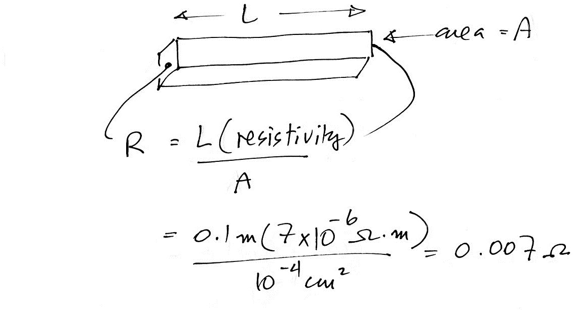
This was a relatively quick problem to work
out. In the first part you were supposed to
calculate the resistance between the ends of a 10 cm
long piece of graphite. You're given the
resistivity which is a property of a given
material. The resistance depends on the shape of
the material.
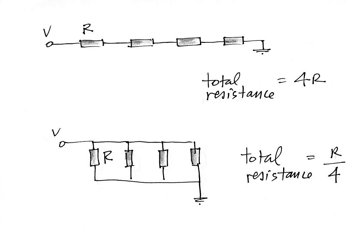
Would the resistance be different if you connected to opposite sides of the piece of graphite? At first glance I would have said no, the electricity is flowing through the same total amount of resistive material. But the mathematics shows otherwise
The resistance in this configuration is lower. To get a physical picture of why this is the case you can imagine electrical current running through several resistors connected in series or in parallel. It's the same total amount of resistive material but the total resistance in the two situations is different.
5. The figure below shows the main features:
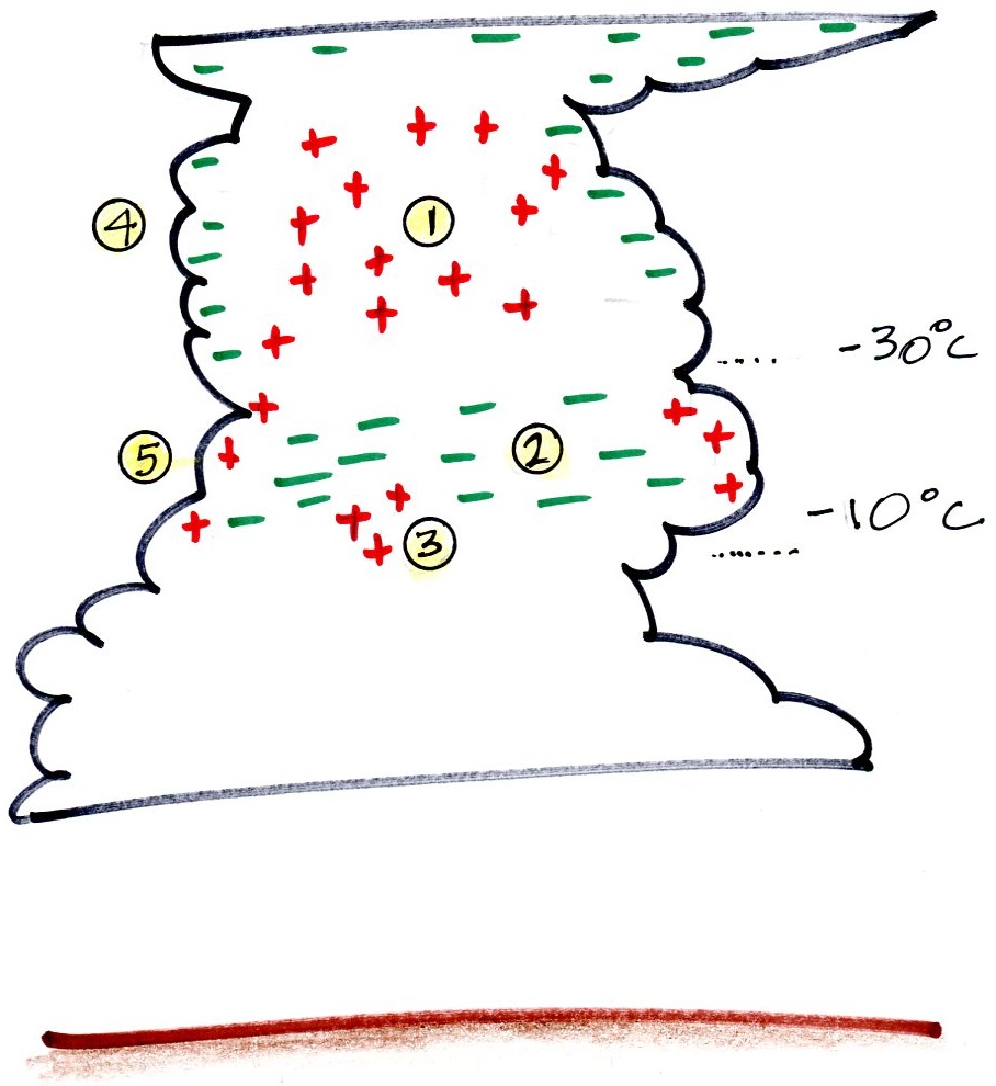
(1) is the main positive charge center. The main negative charge center (2) is more of a layer that seems to always be found between -10 C and -30 C. Smaller volumes of positive charge (the so called lower positive charge centers) are found at (3) in the figure below the main layer of negative charge.
The Reynolds, Brook, Gourley non-inductive electrification process is capable of explaining all three of these features (the figure below comes from the Feb. 18 class).
Would the resistance be different if you connected to opposite sides of the piece of graphite? At first glance I would have said no, the electricity is flowing through the same total amount of resistive material. But the mathematics shows otherwise
The resistance in this configuration is lower. To get a physical picture of why this is the case you can imagine electrical current running through several resistors connected in series or in parallel. It's the same total amount of resistive material but the total resistance in the two situations is different.
5. The figure below shows the main features:
(1) is the main positive charge center. The main negative charge center (2) is more of a layer that seems to always be found between -10 C and -30 C. Smaller volumes of positive charge (the so called lower positive charge centers) are found at (3) in the figure below the main layer of negative charge.
The Reynolds, Brook, Gourley non-inductive electrification process is capable of explaining all three of these features (the figure below comes from the Feb. 18 class).
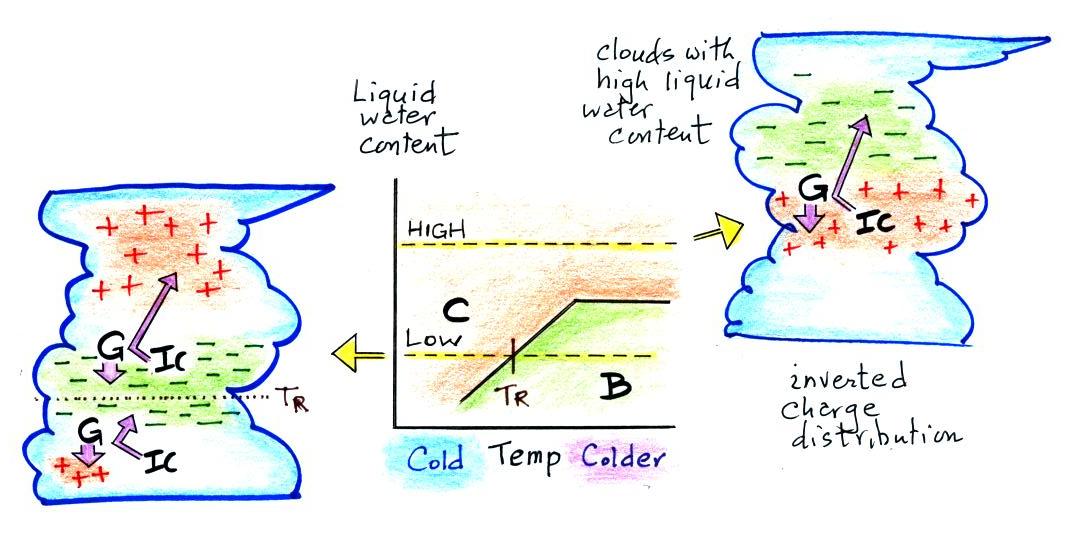
Basically graupel particles
(G in the figure) collide with smaller ice
crystals (IC) in the presence of supercooled water
droplets. Usually the graupel will end up
with negative charge and the ice crystal will be
positively charged. The smaller, lighter ice
crystals are carried up toward the top of the
thunderstorm. At temperatures warmer than TR
(but still below freezing) the polarities are
reversed. This is thought to be responsible
for the lower positive charge centers.
This process is also able to explain the inverted polarity thunderstorms (the cloud at upper right in the figure above) that sometimes are seen in strong storms in the Central Plains with high liquid water contents.
The layers of charge found at the cloud boundaries (points (4) and (5) in the earlier figure), screening layers, form when currents flowing toward or away from the cloud encounter an abrupt change of conductivity at the edges of the cloud (much lower conductivities inside the cloud).
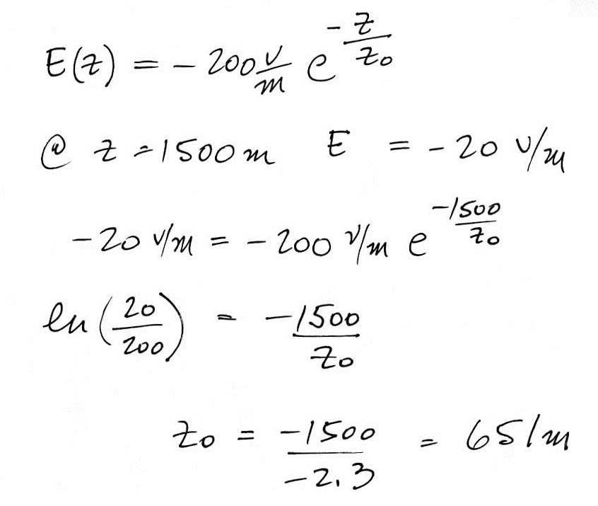
6. We're given an expression for E(z) and first need to determine the value of zo
This process is also able to explain the inverted polarity thunderstorms (the cloud at upper right in the figure above) that sometimes are seen in strong storms in the Central Plains with high liquid water contents.
The layers of charge found at the cloud boundaries (points (4) and (5) in the earlier figure), screening layers, form when currents flowing toward or away from the cloud encounter an abrupt change of conductivity at the edges of the cloud (much lower conductivities inside the cloud).
6. We're given an expression for E(z) and first need to determine the value of zo
Then we will use the
differential form of Gauss' law to determine
the volume space charge density ρ(z)
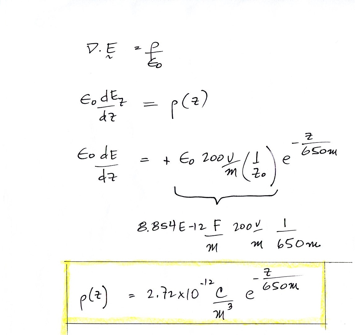
The space charge has
positive polarity.