Friday Mar. 6, 2015

Lightning Channel Current I(z,t)
The E and B fields at a particular distance from a lightning strike depend in a complex way on return stroke current, the current derivative, and, for E fields, on the time integral of the current.  We really don't know what the return stroke current is as a function of altitude and time [ that is, I(z,t) ].  At best we can sometimes measure I(0,t) [i.e. the current at the ground in triggered lightning discharges, for example]

Let's remember that what we are hoping to do is to measure E and/or B and go back and figure out what the return current must have been.  In order to do that we will need to make some assumptions or put some constraints on the return stroke current.  We will need a lightning return stroke "current model."

We can roughly classify current models into 3 groups:

1.  Sophisticated plasma-fluid-dynamics models that try to realistically determine the actual physical conditions in a lightning channel (temperature, electron density, pressure, and other electrical and fluid properties).  This type of approach is beyond the scope of this class.  (see M.N. Plooster, "Numerical Simulation of Spark Discharges in Air" and "Numerical Model of the Return Stroke of the Lightning Discharge" for examples of this type of approach)

2.  Because the lightning return stroke current begins at (or near) the ground and travels upward along a conducting channel, many researchers treat the return stroke as a voltage or current pulse traveling along a transmission line with distributed resistance, inductance, and capacitance. (see for example P.F. Little, "Transmission Line Representation of a Lightning Return Stroke" and G.H. Price and E.T. Pierce, "The Modeling of Channel Current in the Lightning Return Stroke")

We will adopt more of an engineering or empirical approach
3.  We will assume a functional form for I(z,t), calculate the E and B field that such a current would produce, and then compare the calculations with field measurements (often made at two distances from the return stroke).  We will then adjust I(z,t) or other model parameters such as propagation speed to get the best agreement between calculated and measured fields.


We'll mostly just discuss two well know current models: the Bruce-Golde and the Transmission Line models.

Bruce Golde Model


In the Bruce Golde model the return stroke current is assumed to be uniform along the length of the channel.  The current amplitude can change with time but it does so along the entire length of the channel simultaneously.  This is illustrated further in the figure below which shows the height of the return stroke channel and the current distribution along the channel at evenly spaced time intervals t1 through t5.  The width of each vertical bar indicates the current amplitude.  As the current amplitude is changing at the ground with time, current amplitude also changes simultaneously along the entire length of the channel.


The current waveform measured at the ground and at Pt. B above the ground are shown at the bottom of the figure.   It takes time some time before the current reaches Pt. B but from the time onward, the current waveforms measured at the ground and at Pt. B are identical.  Any change in the current at the ground occurs simultaneously at Pt. B.


Here is first an expression for the radiation field component of the electric field (Erad) at a distance D from the lightning stroke.  There are a few tricks involved in this derivation (that we won't worry about) because the current is discontinuous at the tip of the upward propagating return stroke current.  The expression for E can be inverted to give the channel base current as a function of the field (the last equation in the figure above).


Transmission Line Model
In the transmission line model the current waveform measured at the ground is assumed to propagate up the channel without changing shape and at constant speed.  Here's how that is expressed in equation form.


Basically the current value observed at height z at time t is the same as the current seen at the ground at a time (t - z/v) earlier (i.e. the time it took to travel from the ground up to height z).  Again this might be clearer in picture form.


The current waveform measured at the ground propagates up the channel without changing shape or speed.  The same current waveform would be seen at all points on the channel just delayed with respect to the ground.

The radiation field dE produced by a segment dz of channel located at height z above the ground is shown below


Because of the functional form of I(z,t), we can replace the partial derivative with respect to time with a partial with respect to z.


This makes it easy to integrate over z.


H is the height of the return stroke channel.  The first term in brackets is zero at times less than H/v (i.e. before the return stroke tip reaches the top of the channel).


You couldn't ask for a simpler relationship between E and I (or dE/dt and dI/dt).
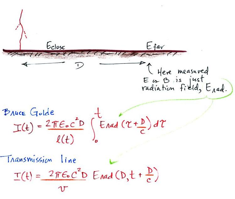
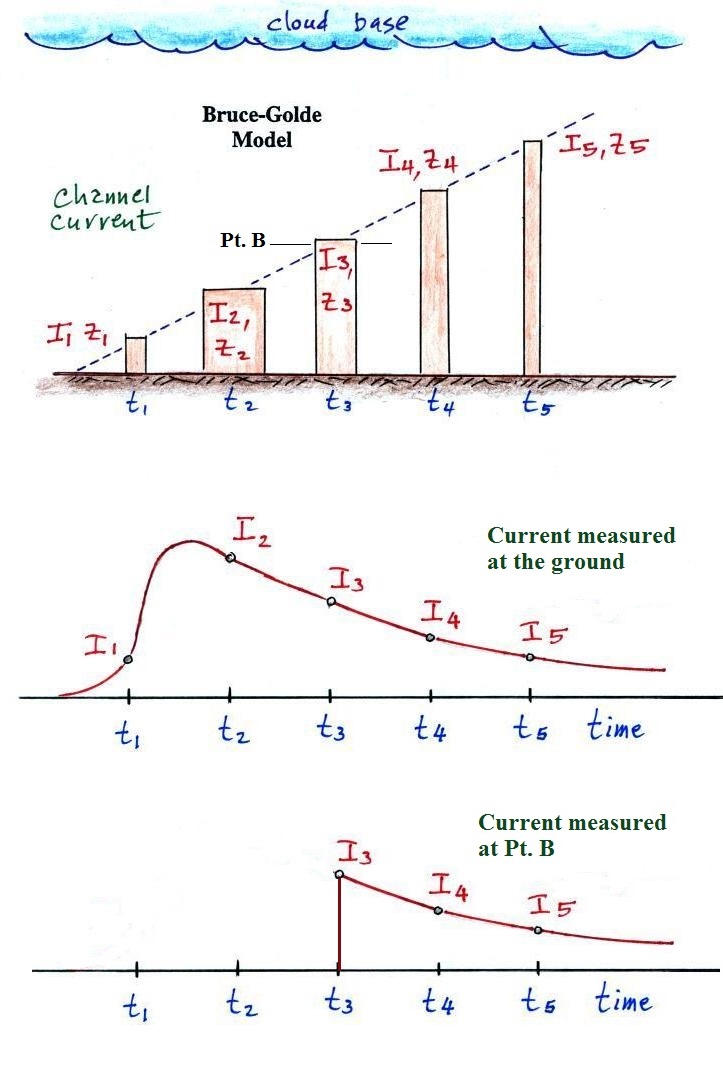
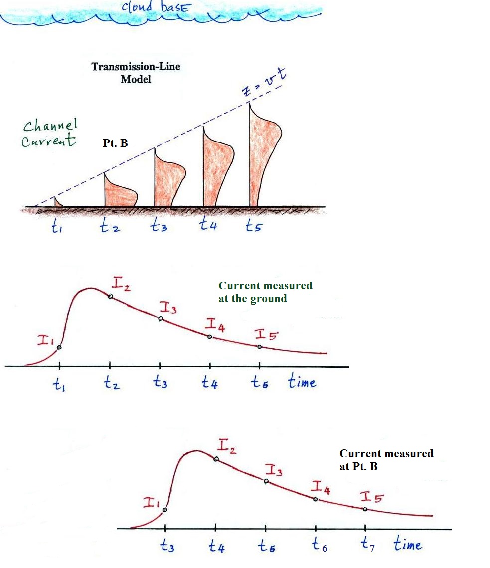
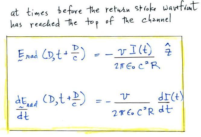
Erad has the same shape as the current waveform measured at the ground.  Ditto for dErad/dt and dI/dt.

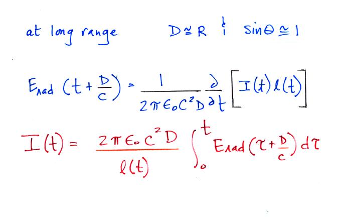
These expressions are widely used to estimate Ipeak and peak values of dI/dt from measured Erad and dErad/dt.

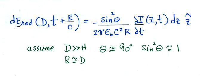
Note both the peak I and peak dI/dt occur when the tip of the upward moving return stroke current waveform is close to the ground.  This assumption that the return stroke channel is straight and vertical might not be too bad at this point.  The assumption that sin θ   = 1 is also not too bad.


Experimental Test

Now we'll look at an experimental test of the Bruce Golde (BG) and Transmission Line (XL) models.  We'll also look at a second, different experimental test of the Transmission Line.  But not until our next class.


Simultaneous measurements of electric and magnetic fields were made at 2 stations: one close to and the other far from the strike point.  The far field measurements (which are just radiation fields and don't contain any induction or electrostatic fields) were used to determine the return stroke channel current, I(t), using of the two equations above.  Then both near and far fields were calculated and compared with the actual measurements at the two sites. 

Here are some of the results from the tests. 
In this case the distant station (the Kennedy Space Center, Florida) was 200 km from the lightning strike point, the close station (Gainesville, Florida) was only 2 km away.  These data are from  "Lightning Return Stroke Models," by Y.T. Lin, M.A. Uman, and R.B. Standler.


Point 1.  The experimental tests used only the fields from subsequent strokes because, without branches, they are closer to the model assumptions that the lightning channel is straight and vertical.  A constant return stroke propagation speed was assumed and the value was adjusted to give the best fit between measured and computed fields.

Point 2.  Note first the measured distant E radiation field is labeled "Data" on the graph.  This field is used in the Bruce Golde (BG) and Transmission line (XL) models to derive the return stroke current I(z,t) (the derived currents are shown at Point 4).  Then the E radiation fields are computed using both the BG and TL currents.  You can see for the distant fields, the agreement is pretty good but not perfect.  In particular the XL calculated field never goes below zero.

Point 3.  The derived currents were then used to compute the E and B fields at the closer station.  The calculated fields were then compared to the measured fields.  The agreement wasn't particularly good.

Point 4.  The derived currents are plotted.  The XL model current waveform is too narrow and is unrealistic.


An additional set of test results (the lightning strike was 9 km from the measuring site at the Kennedy Space Center and 200 km from the measuring station at the University of Florida in Gainesville).


A return stroke velocity was determined for each set of near and far E and B field measurements (the velocity value was the one that provided the best fit between measured and calculated fields).  The velocity values derived for the BG model are shown in the top graph and appear to be distance dependent (distance from the close station to the lightning strike point).  That is a physically unreasonable result.  The velocities derived for the TL model appear in the bottom plot.  The values are more reasonable; perhaps a little lower than the 1 x 10⁸ m/s commonly assumed for return strokes but at least they do not appear to vary with distance.


Here are the peak current values derived for both the TL and BG models.  In both cases peak current values appear to be distance dependent which is not realistic.  Many of the TL peak currents are too large.  First return stroke peak currents are typically about 30 kA.  Subsequent stroke peak currents are usually less.  Some of the TL peak currents in the plot above exceed 100 kA.

Neither the transmission line or the Bruce-Golde did a very good job of reproducing the measured fields, particularly at close range.  The researchers that conducted these experimentals tests made some changes to the assumed return stroke current.  In particular they found that 3 current components were needed to better reproduce the near fields: a breakdown current, a corona current and a uniform current.  (source: Uman, M.A., The Lightning Discharge, Academic Press, Orlando, 1987, see also the Lin, Uman, and Standler (1980) reference mentioned earlier).


We won't discuss this further in this class as we'll mostly be interested in estimating peak I and peak dI/dt values from measurements of radiation fields.  And in that case it looks like the transmission line model does a pretty good job.  We'll look at this more recent test of the transmission line model in our next class.