Friday Jan. 30, 2015


Homework Assignment #2
A new, 2 problem, homework assignment was handed out today.  Rather than making it due next Friday, I decided to make it due a week from Monday (Feb. 9).

The first problem involves determining the field at the surface of a flat conducting plane produced by a charge positioned overhead. 
You might remember having used the "method of images" to solve this problem in an electricity and magnetism course.


The situation that you'll be solving in the homework is shown at left in the figure above (the earth's surface is the conducting plane).   A thunderstorm is often represented by spherical centers of positive and negative charge located above each.  It's the same problem; there are two points charges in this case and one is positioned a little higher than the other.   Most cloud-to-ground discharges carry charge from the lower negative charge center to ground.   You can view this as + ΔQ having been added to and neutralizing some of the charge in the negative charge center.   Q in the homework problem is replaced with
+ ΔQ and you determine  ΔE and the ground rather than E.  An intracloud discharge shown above at right neutralizes charge in both the positive and negative charge centers.

In the second question you're given functions for the change in the fair weather electric field versus altitude between the ground and 30 km altitude.  The expressions fit some measured data fairly well.  The homework problem asks you to determine the potential difference between the ground and 30 km altitude.


Fast and slow E field antennas, passive and active integrators
Next a little more information about the fast and slow E field antennas that we discussed in class on Wednesday.


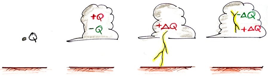
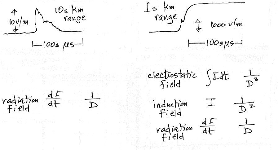
First here are a couple of sketches of the kinds of E fields you might see from a lightning strike to the ground (a return stroke) at relatively far range (10s of kilometers) at left and closer range (a few kilometers away) at right. 

The close field at right is made up of several components (and we'll look at all of this in more detail later in the class)
(i)  an electrostatic field that is proportional to the integral of the return stroke current.  This field component is slow to develop because of the integral over time.  Also the 1/(distance)3 dependence means it weakens very quickly with distance The integral of current over time is just charge.  This is the field that you are able to monitor with a field mill.
(ii) a field that depends on current and decreases with a 1/(D)2dependence
(iii) the radiation field depends on dI/dt.  It peaks early in the discharge and falls off slowly with distance.
You could use both fast and slow E field antennas to study this close field

The more distant field consists of just the radiation field term.  A fast E field antenna alone is all you would need to measure and record a distant field like this.


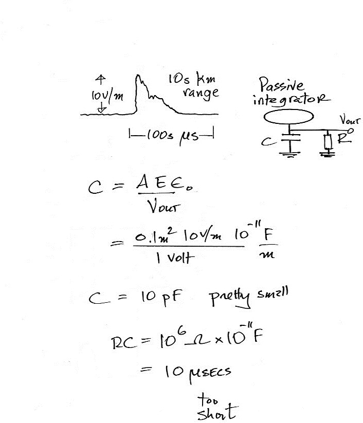
Here we're estimating the value of the capacitance needed in a passive integrator to produce an output voltage of 1 volt (we assume the antenna area is 0.1 m2).  C would need to be 10 pF.  That's pretty small, stray capacitance in the antenna itself could be several times that.  Then when we need to connect to some kind of measuring or recording device like an oscilloscope.  We'll assume that has an input impedance of 1 M Ω The resulting decay time constant, 10 μs, is too short. 

In a case like this the antenna needs to be connected to an active integrator as shown below.


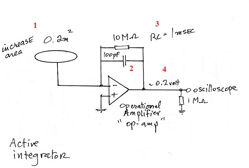
We've made the antenna area a little larger to increase the signal (Pt. 1).  Instead of 10 pf, we've used a 100 pF capacitor in the feedback look of the op-amp (Pt. 2).  The decay time constant is determined by the produce of R and C in the feedback loop (Pt. 3) and doesn't depend on the input impedance of the oscilloscope.  A 10 V/m E field signal would produce a 0.2 volt output signal in this case.

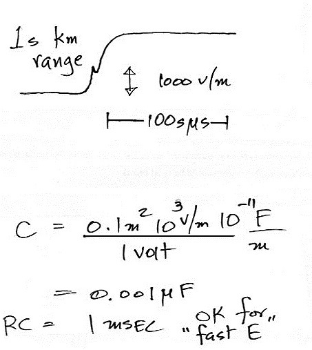
A passive integrator circuit would work for the closer discharge.


Because of the larger E field signal, a larger capacitor can be used.  The decay time constant in this case is 1 ms, which is suitable for a fast E antenna system (we've assumed a 1 M Ω oscilloscope input impedance).

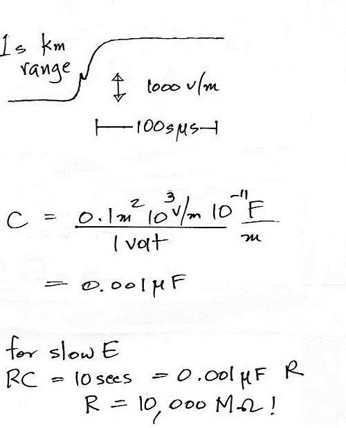
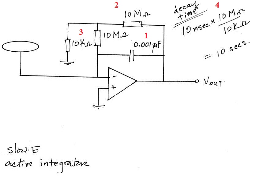
A slow E field antenna system would be needed to faithfully record the longer duration field variations in these nearby discharges. 


A much larger resistance is needed across the integrating capacitor to increase the decay time to 10 seconds.  You can find resistances this large.  But when the passive integrator is connected to a recorder the 1 M Ω input impedance of the recorder in parallel with the 10,000 M Ω resistor would lower to overall resistance to about 1 M Ω.  An active integrator circuit is needed here also.


We've used the same 0.001 μF integrating capacitor (Pt. 1)with a 10 M Ω resistor in parallel (Pt. 2).  Two additional resistors have been added to the circuit (Pt. 3).  The effect they have is to multiply the 10 ms decay time by a factor of 1000 resulting in a 10 second decay time.  That's a very reasonable value for a slow E antenna.

Don't worry about all the circuit details.  I've included them just to illustrate some of what needs to be considered when designing these E field antenna systems.

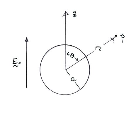
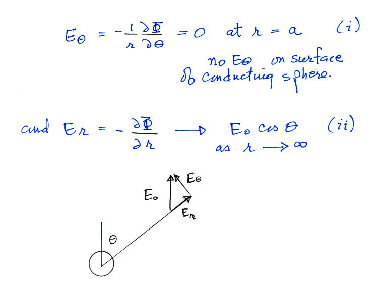
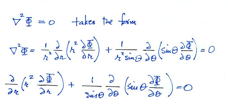
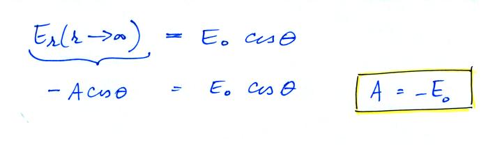
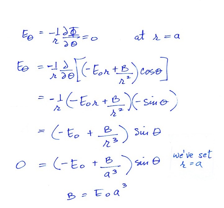
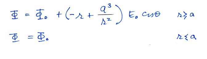
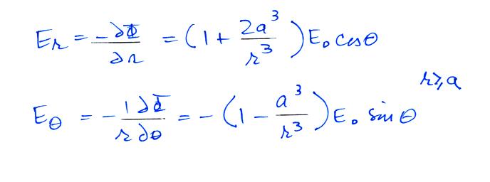
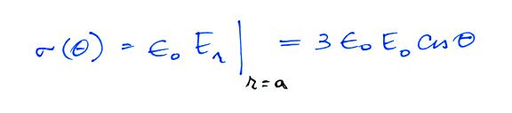
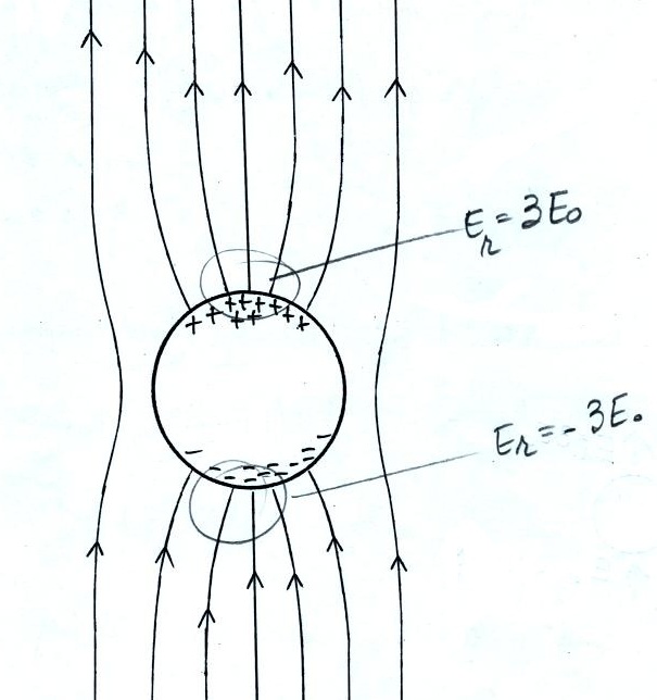
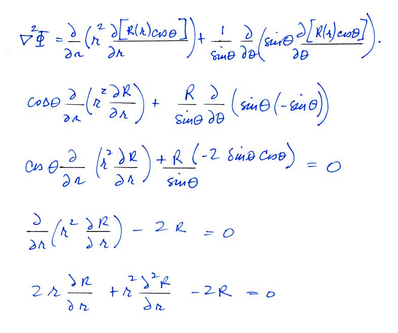
Conducting Sphere in a Uniform Electric Field
Here's another problem you probably worked out in an electricity and magnetism class.  We're going to determine how an initially uniform electric field, Eo, is distorted by the presence of an uncharged conducting sphere.  Charge is induced on the surface of the sphere and it moves around until the field inside the sphere becomes zero.   The sphere distorts the field in such a way that the field lines are everywhere normal to the surface of the conductor.   

We'll use spherical polar coordinates and place the origin of our coordinate system at the center of the sphere,


There is azimuthal symmetry, so the potential and the electric field depend on r and θ  only.  We can proceed to solve Laplace's equation for the potential, Φ, subject to the following boundary conditions


(i) There is no   component at the surface of the sphere, just an r component that is perpendicular to the surface.
(ii) The second condition is just that as you move well away from the sphere the r and
θ components of the field add up to produce Eo pointing in the z direction

In the spherical coordinate system


Assuming the variables are separable, we try a general solution of the form:

Just looking at the boundary condition (Eqn. (ii)), we simply try a T(θ) function of the form


Now, inserting this into our original differential equation, we find

Some of the missing details are appended at the end of this section.

Now, let's try a solution to the R equation of the form


When we substitute this into the differential equation above we get


Now a general R solution will be of the form


and

Where A and B must be determined from the boundary conditions.

Now,


applying boundary condition (ii) as r goes to infinity


next we make use of the other boundary condition.  We need to find the
θ component of the field and then set r = a


and our potential function is now


with this Φ our electric field components are:


and the surface charge density is


Our main interest in this result is that the sphere has enhanced the value of the ambient field at the top and bottom surface of the sphere by a factor of 3.


This figure gives you a rough idea of how the field is changed in the vicinity of the sphere.  E field lines must intersect the sphere perpendicularly. The field is amplified by a factor of three at the top and bottom of the sphere.


Enhancement of fields by conducting objects is an important concern.  In some cases (we'll look at an example or two next week) the enhanced field is strong enough to initiate or trigger a lightning discharge.

Some of the details of one of the earlier calculations are shown below: