Monday Feb. 9, 2015
Homework
Assignment #2 was collected today. I should have
another assignment ready by Wednesday.
I
didn't have a chance to discuss the ionization type smoke
detector or the Nu Klear Fallout Detector in class last
Friday so we did that today. You'll find the
discussion in the Friday Feb. 6 notes. There's also a
link to a good video
explanation of the operation of the smoke detector.
We first need to finish up an example that we didn't have
time for in our last class. It deals with what happens
along an air-cloud boundary where there is an abrupt change
in conductivity.
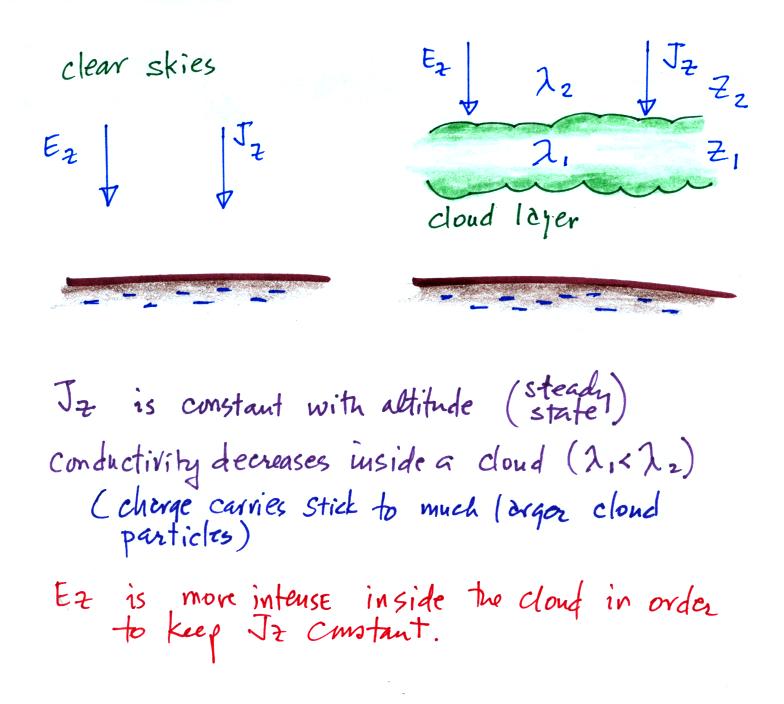
Conductivity inside a cloud is lower than in the air outside
a cloud. This is because the small ions attach to much
larger and much less mobile cloud particles (water droplets
or ice crystals). The E field must become stronger
inside the cloud so that the current density (the produce of
conductivity and electric field) stays the same inside and
outside the cloud. We'll see that layers of charge
build up on the top and bottom surfaces of the cloud.
We'll try to estimate how much charge is necessary along the
upper surface of the cloud layer.
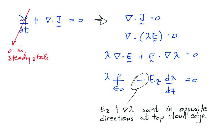
We
don't
really know Ez. The current density,
Jz, on the
other hand is constant with altitude and we assume we know
how conductivity changes as you move across the cloud-air
boundary.
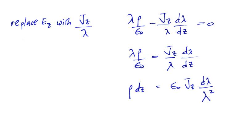
We
can
integrate this equation
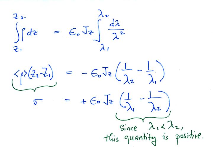
So
we conclude a layer of positive charge builds up on the top
edge of the cloud. In a similar kind of way you could
show that a layer of negative charge would build up on the
bottom edge of the cloud.
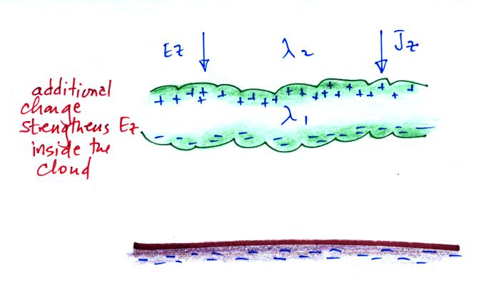
The effect of these two layers of cloud is to intensify the
field inside the cloud. The product of higher field
times lower conductivity inside the cloud is able to keep
the current density equal to the current density outside the
cloud.
Screening layers that form along the edges of a thunderstorm
effectively mask the main charge centers inside the cloud.
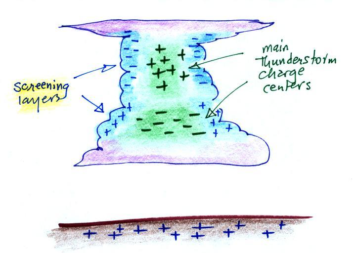
One of the consequences of this is that it makes it
difficult to use measurements of E field at the ground to
estimate how much charge builds up in the main charge
centers inside the cloud. We will find that if you use
sudden abrupt changes in electric field, ΔE
measurements, you can determine the amount and
location of charge neutralized during lightning
discharges. The abrupt field change occurs quickly
enough that there isn't sufficient time for the charge
screening layers to rearrange themselves and mask the field
change.
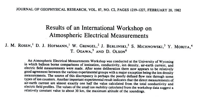
The next several figures show measurements of fair weather
conductivity, electric field, and current density made
during a field experiment in 1978 in Wyoming.
Simultaneous measurements were made with a variety of
different instruments from different research groups.
Instruments were carried up to about 30 km altitude by
balloon and measurements were made on the ascent and often
during the descent. Here's a link to the full article
(pdf file).
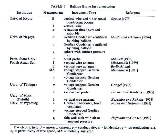
The
list below gives you an idea of the electrical parameters
that were measured and the various types of sensors that
were used.
Measurements
of
conductivity versus altitude made on two different days are
shown in two graphs below.
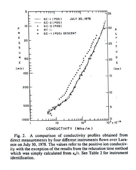
Conductivity values range from about 5 x 10-14
mhos/m at 2 km or so above the ground to about 1000 times
higher near 30 km. Note that conductivity is plotted
on the x-axis on a logarithmic scale. The 10 - 30 km
portion of the graph appears pretty linear implying
conductivity is decreasing exponentially with
altitude.
The conductivity values are from just the positively charged
small ions. The notation "GC" in the figure refers to
"Gerdien Condenser." The
cylindrical capacitor discussed in the last lecture would be
an example of a Gerdien
condenser type instrument. Conductivity was estimated
using the Isignal/V slope
method described in our last lecture (σ is used in
the article instead of λ).
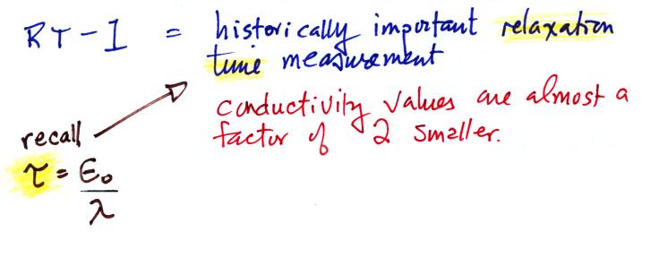
All of the measurements are in good agreement with the exccption of the relaxation time
method. This is just the decay time constant we
derived in a previous lecture.
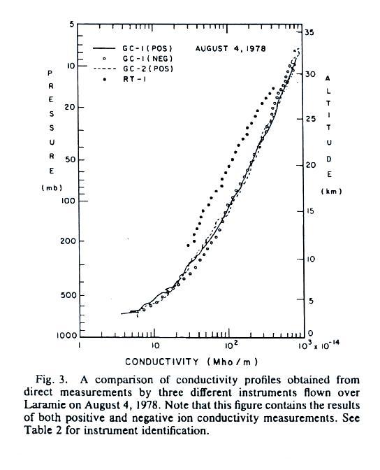
A
second set of conductivity measurements. These include
both positive and negative small ions.
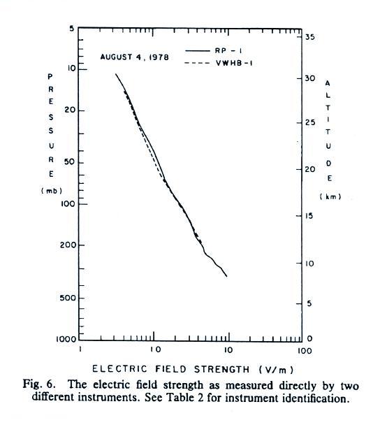
The
next
two plots show measurements of electric field versus
altitude (the same two plots were on the homework assignment
that was collected today).
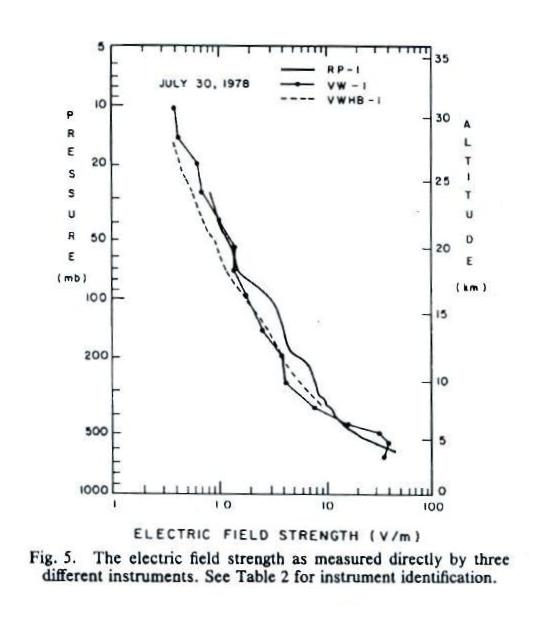
E field values decrease from a few 10s of volts/meter 2 or 3
km above the ground to less than 1 V/m near 30 km (note:
the x-axis values are, from left to right, 0.1, 1.0, 10 and
100 V/m).
The
next plot shows the vertical profile of current density, Jz. Measurements from two
different days are plotted together.
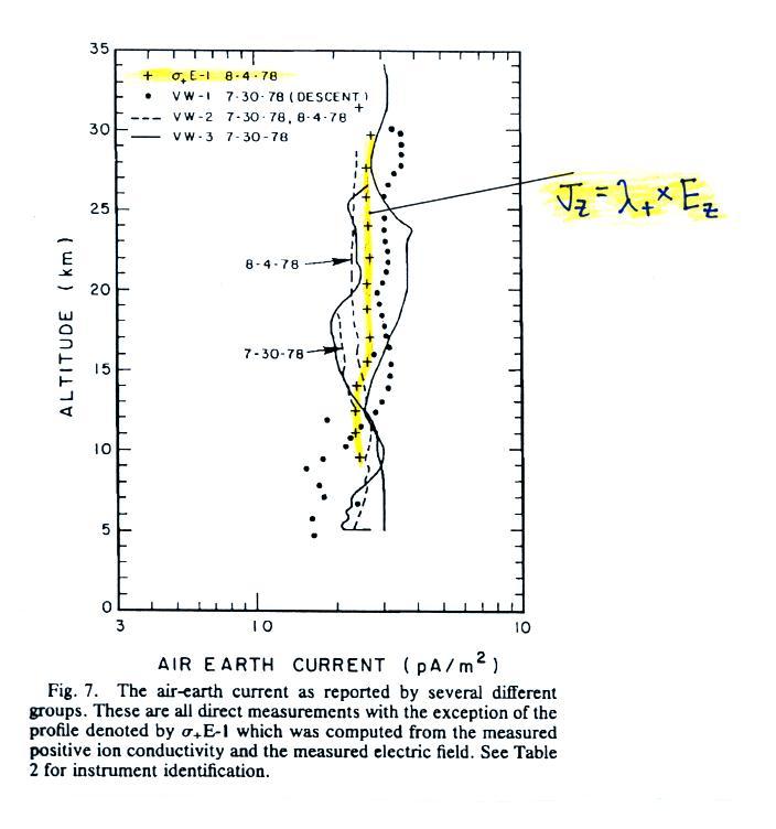
Note first of all that current density does stays fairly
constant with altitude something we expect under steady
state conditions (the x-axis labels, from left to right, are
0.1, 1.0 and 10 pA/m2).
The
yellow curve is the product of electric field and positive
small ion conductivity, all the others are measurements of Jz. You
would expect the measured Jz
(which includes both positive and negative charge
carriers) to to be roughly
twice the positive conductivity times electric field, but it
isn't. For that reason the
data above was not included in the handout distributed
in class.
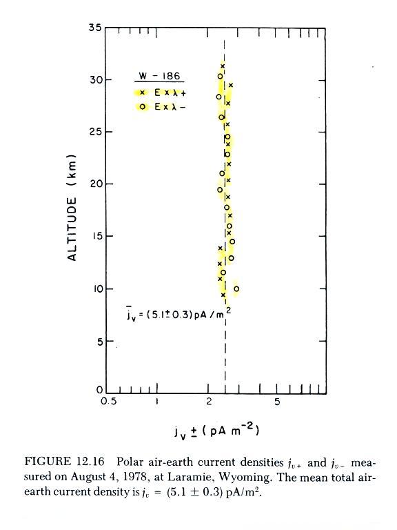
The problem appears to have been corrected in the plot below
which is a reanalysis of the Wyoming data. The plotted
points are conductivity (positive and negative polarity)
times measured electric field. The plotted values
cluster around a value of about 2.5 pA/m2
(note again how uniform Jz
is with altitude). Measured Jz
was about twice this, about 5.1 pA/m2.
The next graph summarizes measurements from a different
field experiment conducted in the North Atlantic ocean.
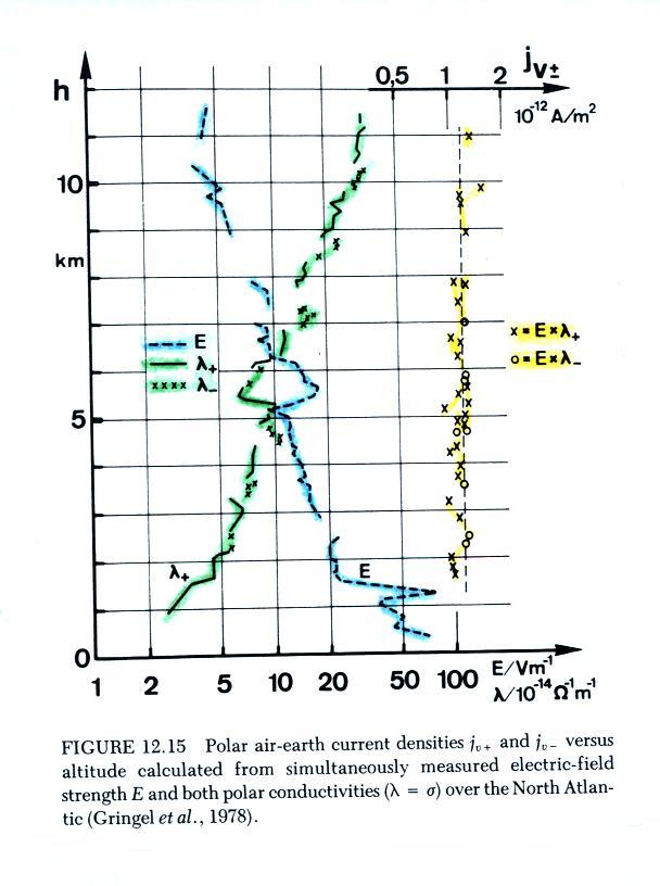
The
plot
shows vertical profiles of E field (highlighted in blue),
measured positive and negative conductivities (green), and
the calculated current density (in yellow, the product of
positive and negative conductivity and measured electric
field). The calculated current density values are
clustered around 1.25 pA/m2,
the measured total current density was about twice that,
2.35 pA/m2.
The last two figures above from W. Gringel,
J.M. Rosen, ande D.J. Hofmann,
"Electrical Structure from 0 to 30 km Kilometers," Ch. 12 in
The Earth's Electrical Environment, National Academy
Press, 1986. (available online at www.nap.edu/books/0309036801/html/)
Now the main part of today's class, we'll start to look at
how small ions are created. Small ions are the mobile
charge carriers that give the atmosphere it's
conductivity. First something must ionize air
molecules
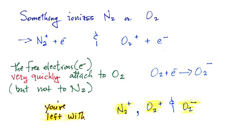
Then water vapor molecules cluster around the ions to create
"small ions." Water molecules have a dipole structure
as shown below.
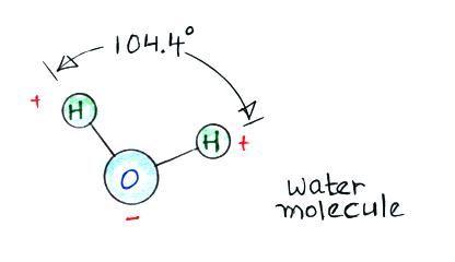
The oxygen atom carries excess negative charge and the
hydrogen atoms positive charge. Because of this the
water vapor molecules orient themselves differently around
the oxygen and nitrogen ions. Conceptually this would
look like
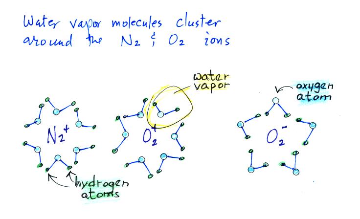
More
water
vapor molecules are able to surround the positive ions so
they are bigger and have slightly lower electrical mobility
than the negative small ions.
The next figure summarizes the processes that ionize air.
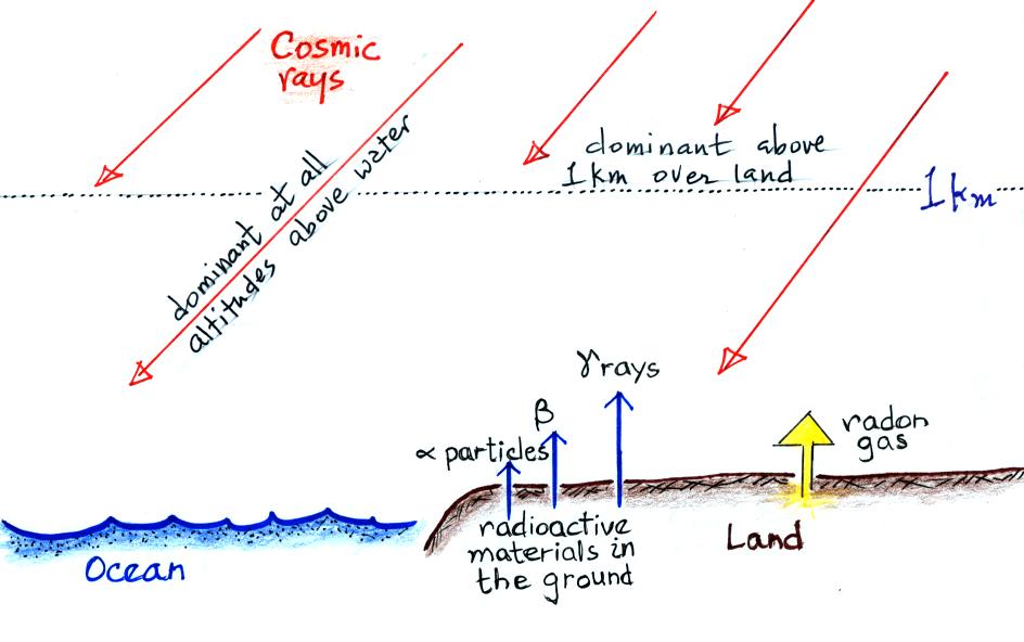
Radioactive materials in the ground emit alpha and beta
particles, and gamma rays. Alpha particles (i.e. a
helium nucleus consisting two protons and two neutrons) are
a strong source of ionization but only in the first few cm
above the ground. Beta particles (electrons) ionize
air in a layer a few meters thick. The effects of
gamma radiation extend of 100s of meters. Cosmic rays
are the dominant source of ionization everywhere over the
ocean and above 1 km over land.
The table below, not shown in class, gives an idea
of how far these different types of radiation can travel
above the ground and also typical ionization rates (ip stands for "ion pairs"). (from
Chapter 11 in "The Earth's Electrical Environment," National
Academy of Sciences, 1986 )
|
emission type |
range of travel |
ionization rate [ ip/(cm3
sec) ] |
|
alpha particles |
only a few cm above the ground |
not well known |
|
beta particles |
a few meters above the ground |
0.1 to 10 |
|
gamma rays |
100s of meters above the ground |
1 to 6 |
|
radon |
depends on atmospheric conditions |
1 to 20 at 1-2 m above ground |
|
cosmic rays |
1 to 2 ip/(cm3
sec) near the ground |
|
In addition to being a source of atmospheric ionization,
radon is a signficant health
hazard and is the 2nd leading cause of lung cancer after
cigarettes. Here are links to articles concerning
radon from the World Health Organization,
Wikipedia, and the Environmental Protection Agency.
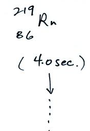
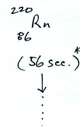
The following table shows a portion of the decay series that
ultimately yield isotopes of radon.
|
|
|
|
|
|
|
|
|
|
|
|
|
|
|
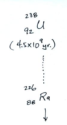
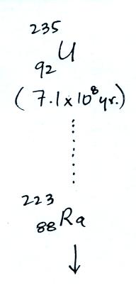
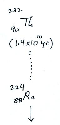
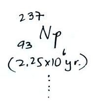
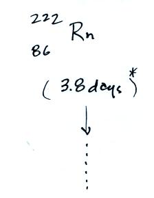
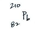
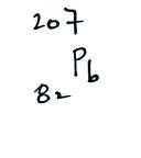
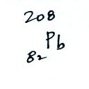
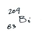
Because
of its relatively short half life compared to the age of the
earth, all the Neptunium in the ground has decayed
away. Two isotopes of radon (Rn-222 and Rn-220) have
half lives long enough to be able to diffuse out of the soil
and into the air.
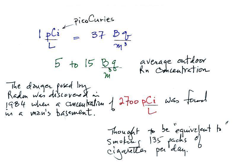
The article from the World
Health Organization gives a typical outdoor
radon concentration of 5 to 15 Becquerels/m3
(Bq/m3
- 1 Becquerel is one disintegration per second
). This is something you could measure with a detector
of some kind, maybe a Geiger counter. This is not
really a concentration, rather a decay rate (dN/dt in the
equation below). We can do a calculation to see what
this implies in terms of radon concentration and ion pair
production rate.
The rate at which a radioactive material decays is described
by the following equation
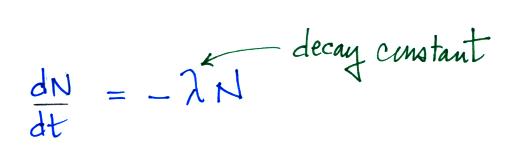
(note: so far in this
course we have used λ to represent linear charge
density, atmospheric conductivity, and now decay
constant).
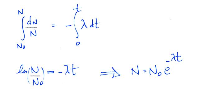
We can solve the equation above to give
It
is
easy to relate the half life, t1/2, and
the decay constant λ
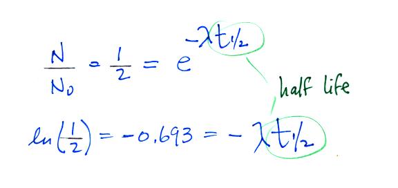
The
Rn-222
isotope has a half-life of 3.8 days.
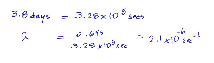
Now that we know the decay constant we'll substitute back
into the decay rate equation to determine the radon
concentration needed to produce an average outdoors decay
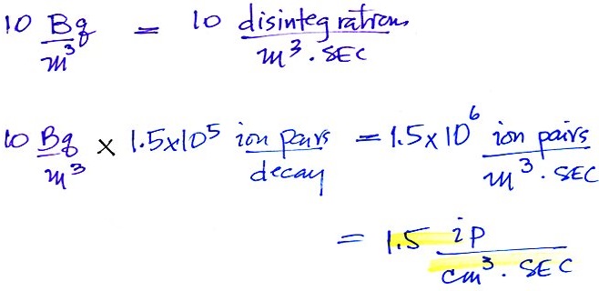
rate of 10 Bq/m3.
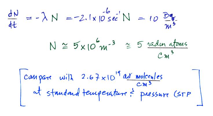
(the number density for air, 2.67 x 10¹⁹ air
molecules/cm3 is sometimes known as Loschmidt's number).
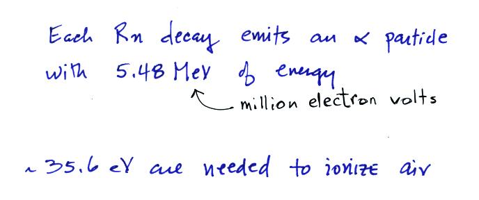
We know the decay constant and now have a typical Rn concentration. Lastly we
can estimate the ionization rate caused by this average
outdoors radon concentration. We need to know how much
energy is contained by the α-particles emitted by
radon and the energy needed to ionize air.
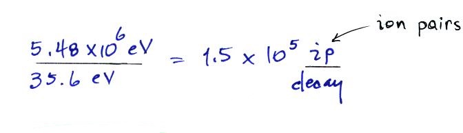
We can divide these two numbers to determine the number of
ion pairs produced by each distintegration.
Then we multiply by the Rn
concentration and the decay constant (which give the decay
rate) to determine the ionization rate.
Radon is a signficant health hazard, causing about 20,000 lung cancer deaths per year in the US. The following information about radon wasn't mentioned in class.
Radon gas decays into solid particles of polonium, lead, and bismuth. The decay series is shown below (source):
- 222Rn, 3.8 days, alpha decaying to...
- 218Po, 3.10 minutes alpha decaying to...
- 214Pb, 26.8 minutes, beta decaying to...
- 214Bi, 19.9 minutes, beta decaying to...
- 214Po, 0.1643 ms, alpha decaying to...
- 210Pb, which has a much longer half-life of 22.3
years, beta decaying to...
- 210Bi, 5.013 days, beta decaying to...
- 210Po, 138.376 days, alpha decaying to...
- 206Pb, stable.
These decay products can attach to dust particles which are
then inhaled and trapped in the lungs. Since the decay
products are themselves radioactive, long term exposure can
ultimately lead to lung cancer. Radon is apparently
the 2nd leading cause of lung cancer in the US after
cigarette smoking.
Radon concentration indoors can build to levels that are
much higher than normally found outdoors. An extreme
case is mentioned below.
You can read more about radon and ways of reducing your
exposure to radon at http://www.epa.gov/radon/