The next several figures show measurements of fair weather
conductivity, electric field, and current density made during a field
experiment in 1978 in Wyoming. Simultaneous measurements were
made with a variety of different instruments from different research
groups. Instruments were carried up to about 30 km altitude by
balloon and measurements were made on the ascent and often during the
descent. Here's a link
to
the
full
article (pdf file).
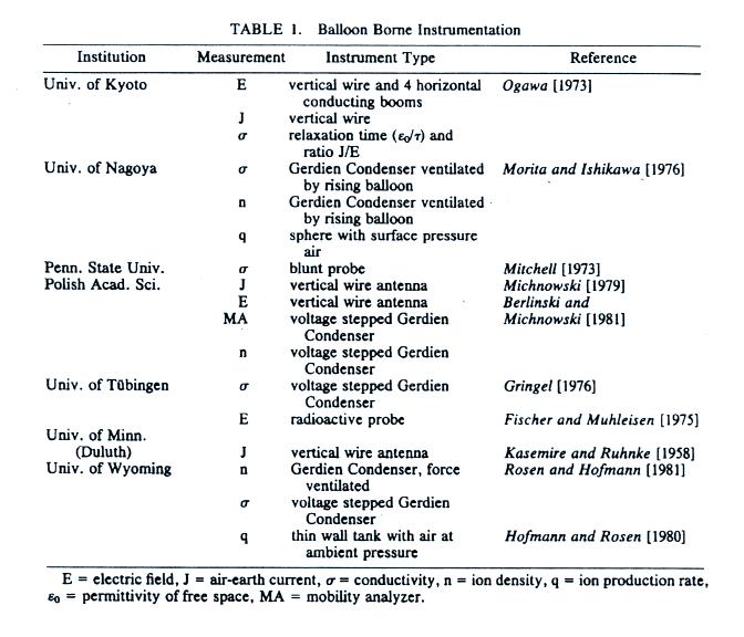
The list below gives you an idea of the electrical parameters that
were measured and the various types of sensors that were used.
Measurements
of
conductivity
versus
altitude
made
on
two
different
days
are
shown
in
two
graphs below.
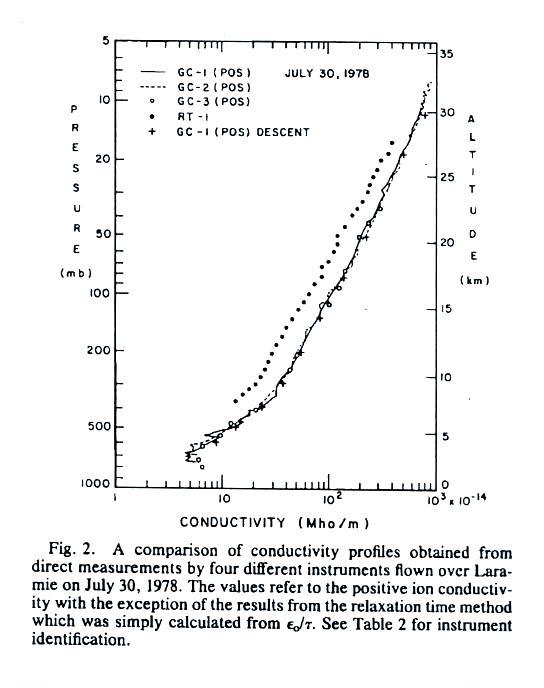
Conductivity values range from about 5 x 10-14 mhos/m at 2
km or so above the ground to about 1000 times higher near 30 km.
The
conductivity values are from just the positively charged small
ions. The notation "GC" in the figure refers to "Gerdien
Condenser." The cylindrical capacitor discussed in the last
lecture would be an example of a Gerdien condenser type
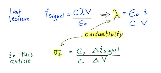
instrument. Conductivity was estimated using the Isignal/V slope
method described in our last lecture (σ
is used in the article instead
of λ).
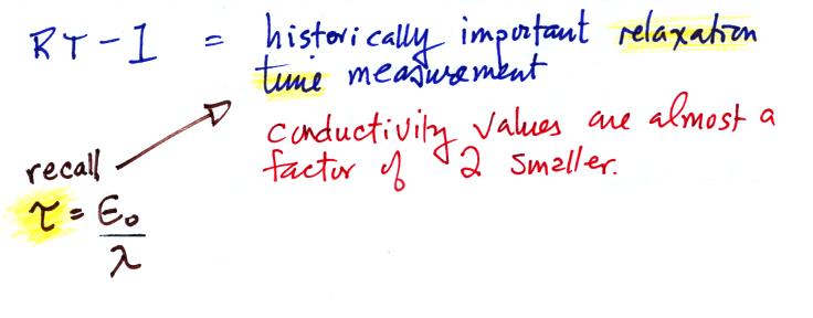
All of the measurements are in good agreement with the exccption of the
relaxation time method. This is just the decay time constant we
derived in a previous lecture.
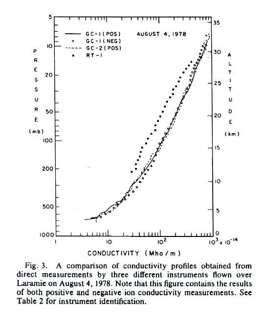
A second set of conductivity
measurements. These include both positive and negative small ions.
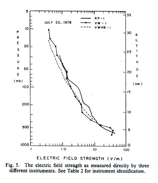
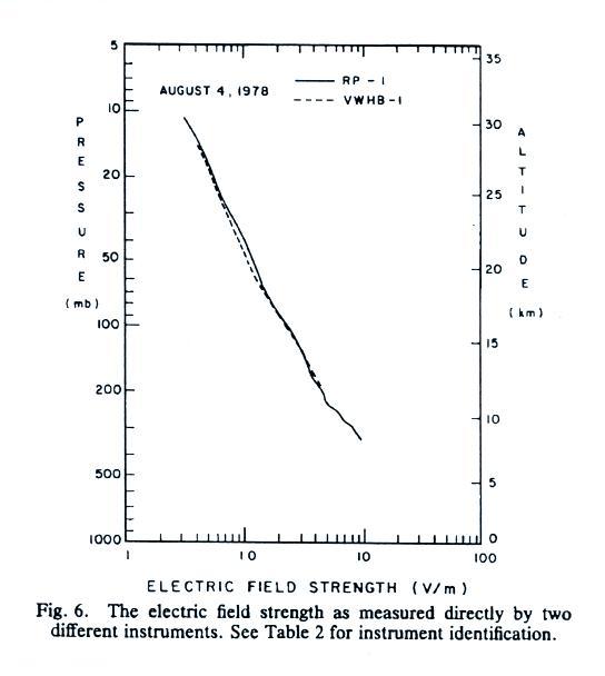
E field values decrease from a few 10s of volts/meter 2 or 3 km
above the ground to less than 1 V/m near 30 km (the x-axis values are,
from left to right, 0.1, 1.0, 10 and 100 V/m).
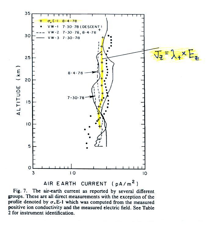
The next
plot shows the vertical profile of current density, Jz.
Measurements from two different days are plotted together.
Note first of all that current density does stays fairly constant
with altitude something we expect under steady state conditions (the
x-axis labels, from left to right, are 0.1, 1.0 and 10 pA/m2).
The yellow curve
is the product of electric field and positive small ion conductivity,
not a measurement of Jz.
You would expect the measured Jz (which
includes both positive and negative charge carriers) to to be roughly
twice the positive conductivity times electric field. The
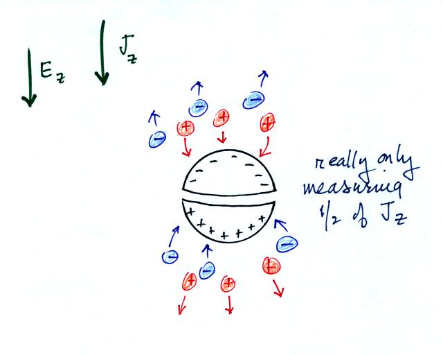
apparent explanation for this descrepancy is shown below (though this
seems like too simple a mistake for the researchers to have made):
One of the Jz
sensors consisted of two conducting hemispheres
insulated from each other. Charge is induced on the two
hemispheres by the ambient electric field. The figure above shows
that the sensor is only capturing half of the charge carries in the
atmosphere and therefore only measuring half of the current density, Jz. There might also
be some uncertainty about the effective
crossectional area of the current sensor.
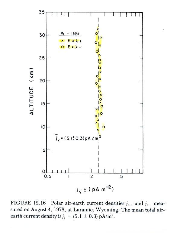
The problem appears to have been corrected in the plot below
which is a reanalysis of the Wyoming data.
The plotted points are conductivity (positive and negative polarity)
times measured electric field. The plotted values cluster around
a value of about 2.5 pA/m2
(note
again how uniform Jz
is with
altitude). Measured Jz
was about twice this, about 5.1
pA/m2.
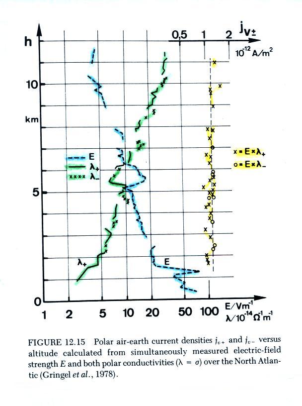
The next graph summarizes measurements from a different field
experiment conducted in the North Atlantic ocean.
The plot shows vertical profiles of
E field (highlighted in blue), measured positive and negative
conductivities (green), and the calculated current density (in yellow,
the product of positive and negative conductivity and measured electric
field). The calculated current density values are clustered
around 1.25 pA/m2, the measured
total current density was about twice
that, 2.35 pA/m2.
Both figures are from W. Gringel, J.M.
Rosen, ande D.J. Hofmann, "Electrical Structure from 0 to 30 km
Kilometers," Ch. 12 in The
Earth's Electrical Environment, National Academy Press, 1986. (available
online
at
www.nap.edu/books/0309036801/html/)
Now the main part of today's class, we'll start to look at how small
ions are created.
Small ions are the mobile charge carriers that give the atmosphere it's
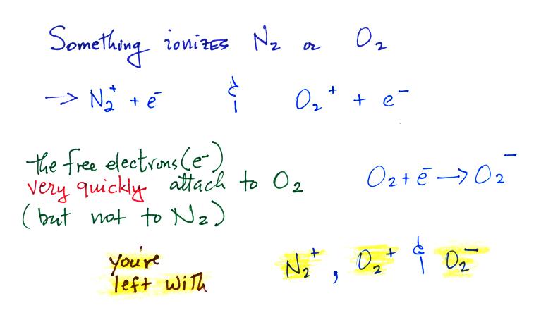
conductivity. First
something must ionize air molecules
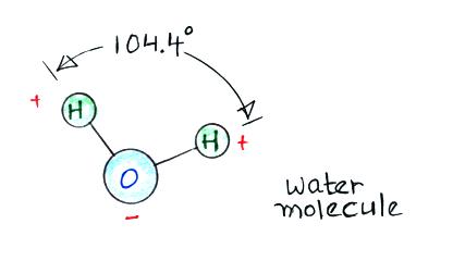
Then water vapor molecules cluster around the ions to create
"small ions." Water molecules have a dipole structure as shown
below.
The oxygen atom carries excess negative charge and the hydrogen atoms
positive charge. Because of this the water vapor molecules orient
themselves differently around the oxygen and nitrogen ions.
Conceptually this would look like
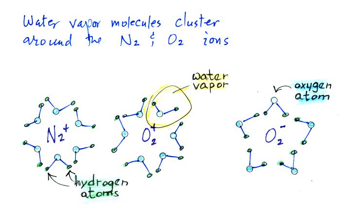
More water vapor molecules are able
to surround the positive ions so they are bigger and have slightly
lower electrical mobility than the negative small ions.
The next figure summarizes the processes that ionize air.
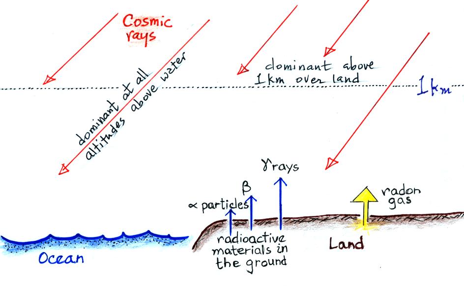
Radioactive materials in the ground
emit alpha and beta particles, and
gamma rays. Alpha particles (i.e. a helium nucleus consisting two
protons and two
neutrons) are a strong source of ionization but only in the first few
cm above the ground. Beta particles (electrons) ionize air in a
layer a few meters thick. The effects of gamma radiation extend
of 100s of meters. Cosmic rays are the dominant source of
ionization over the
ocean and above 1 km over land.
The table below gives an idea of how far these different types of
radiation can travel above the ground and also typical ionization rates
(ip stands for "ion pairs").
(from Chapter 11 in "The Earth's Electrical Environment,"
National Academy of
Sciences, 1986 )
emission type
|
range of travel
|
ionization rate [ ip/(cm3
sec) ]
|
alpha particles
|
only a few cm above the ground
|
not well
known
|
beta particles
|
a few meters above the ground
|
0.1 to 10
|
gamma rays
|
100s of meters above the ground
|
1 to 6
|
radon
|
depends on atmospheric conditions
|
1 to 20 at
1-2 m above ground
|
cosmic rays
|
1
to
2
ip/(cm3 sec)
near
the
ground
|
In addition to being a source of atmospheric ionization, radon is
a signficant health hazard and is the 2nd leading cause of lung cancer
after cigarettes. Here are links to articles concerning radon
from the World
Health
Organization, Wikipedia,
and
the
Environmental
Protection
Agency.
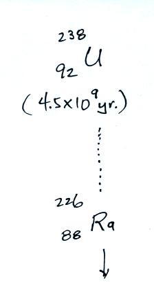
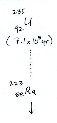
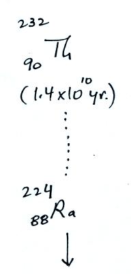
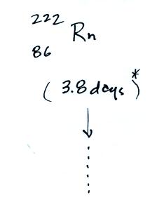
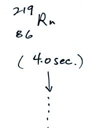
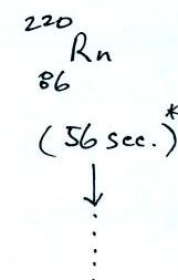
The following table shows a portion
of the decay series that
ultimately yield isotopes of radon.
|
|
|
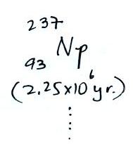
all of the Neptunium in the soil has decayed away..
|
|
|
|
Rn-222,
Rn-219,
and & Rn-220
are sometimes
referred to as
"radon", "actinon",
and "thoron" respectively.
All three are also
known as
"emanatium."
|
|
|
|
|
Because of its relatively short
half like, all the Neptunium in
the ground has decayed away. Two isotopes of radon (Rn-222 and
Rn-220) have half
lives
long enough to be able to diffuse out of the soil and into the
air.
The
article
from
the
World
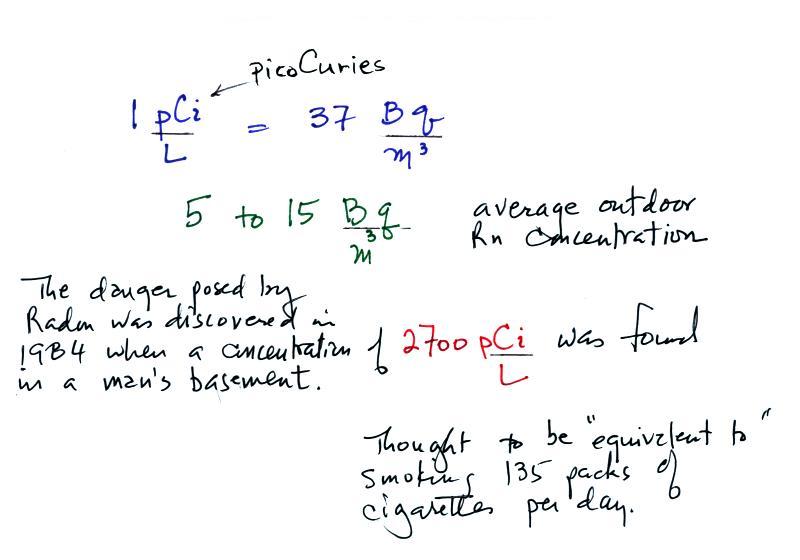
Health Organization gives a typical
outdoor radon concentration of 5 to 15 Becquerels/m3 (Bq/m3 -
1
Becquerel is one
disintegration per second )
. We can do a calculation
to see
what this implies in terms of radon concentration and ion pair
production rate.
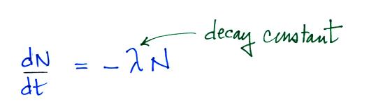
The rate at which a radioactive material decays is described by
the following equation
(so far in this course we have used λ to represent linear
charge density, atmospheric conductivity, and now decay
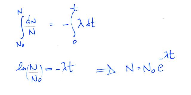
constant). We can solve the equation above to give
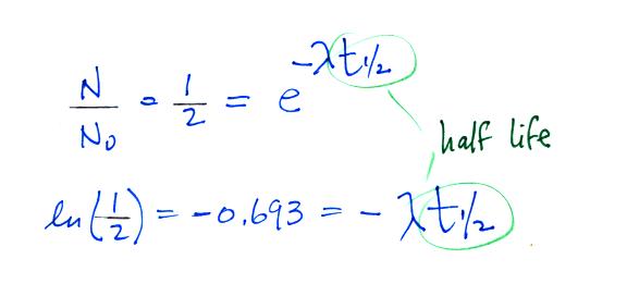
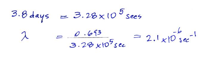
It is easy to relate the half life, t1/2, and the decay constant λ
The Rn-222 isotope has a half-life of 3.8 days.
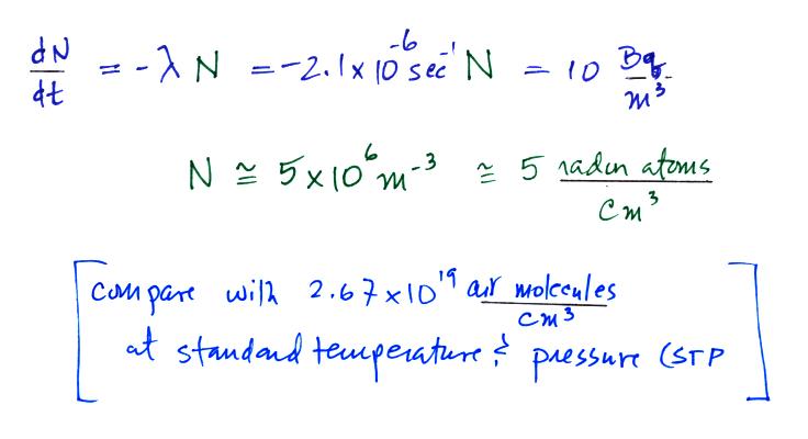
Now that we know the decay constant we'll substitute back
into the decay rate equation to determine the radon concentration
needed to
produce an average outdoors decay rate of 10 Bq/m3.
We know the decay constant and have a typical Rn
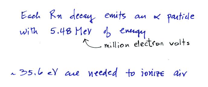
concentration. Next we can estimate the ionization rate caused by
radon. We need to know how much energy is contained by the α-particles emitted by radon and the
energy needed to ionize air.
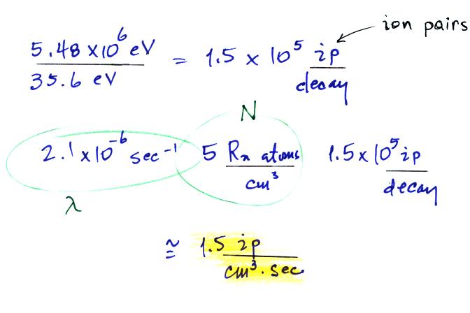
We can divide these two numbers to determine the number of ion pairs
produced by each distintegration. Then we multiply by the Rn
concentration and the decay constant (which give the decay rate) to
determine the ionization rate.
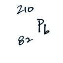
Radon gas decays into solid particles of polonium and lead.
These can attach to dust particles which are then inhaled and trapped
in the lungs. Since the decay products are themselves
radioactive,
long term exposure can ultimately lead to lung cancer. Radon is
apparently the 2nd leading cause of lung cancer in the US after
cigarette smoking.
Radon concentration indoors can build to levels that are much higher
than normally found outdoors. An extreme case is mentioned
below.