Here's an example of a very cleverly designed instrument that has been used to measure electric fields above the ground and inside thunderstorms.  Two metal spheres are attached to and spin around a horizontal shaft.  Everything is carried upward by balloon.  Determining how the two conducting spheres will distort the electric field is a more complex problem than we considered in the last lecture but it has been worked out analytically (don't worry we won't be looking at the details).  You could also work it out numerically or determine the enhancement experimentally.

A rotor causes the two spheres (colored red and green to distinquish between them) to spin as the balloon moves upward.

As the spheres spin, a current will move back and forth between them.  The amplitude of the current will depend on the charge induced on the spheres by the electric field.  The induced charge will, in turn, depend on the intensity of the E field.

The next figure shows an example of data obtained with an instrument like this (it is from a different publication, but a similar instrument was used).


The vertical field swings between large negative and positive values (tens of kilovolts/meter) as the field mill passes through layers of positive and negative charge in a thunderstorm cloud.

Let's use a portion of the E field data to derive an estimate of the average volume space charge density in the lowest layer of charge.

Note that dE/dz is positive on the E field sounding between about 2.7 km and 4.5 km or so.  This coincides with a 1.8 km thick layer of positive space charge.  The slope turns negative between about 4.7 km and 5.1 km where there is a layer of negative charge.  The E field reaches a peak positive value at about 4.6 km, a point that is in between the layers of positive and negative charge.

We can determine the slope of the line highlighted in yellow and use that to determine the average volume space charge density in the layer of positive charge.


The value we obtain (0.27 nC/m3) is in good agreement with the 0.3 nC/m3 value given in the paper.


OK we'll leave the electrostatic stuff behind for a little while and look (again) at currents in the atmosphere.


Currents in the atmosphere and in a wire are compared at the top of the figure above.  A battery voltage drives a current through a wire and resistor in the picture at right.  In the atmosphere, at left, we normally speak of a current density (Amps/square meter) rather than current.  Positive and negatively charged small ions move in response to an electric field and transport charge in air (just the free electrons carry charge in a wire).  We'll refer to this as a conduction current.  Small ions are charged nitrogen and oxygen molecules that are surrounded by water vapor molecules.  We'll look at the creation of small ions in more detail in a later lecture.

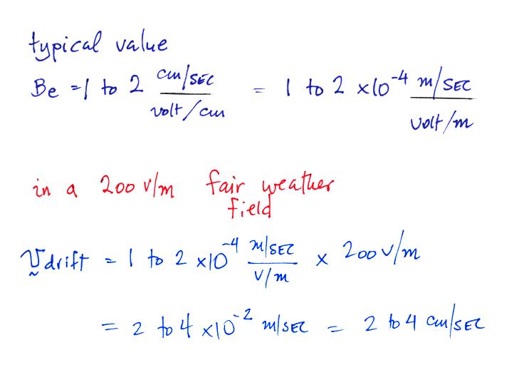
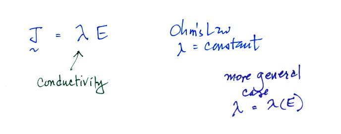
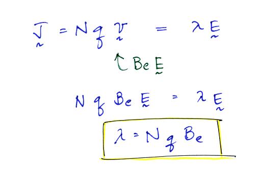
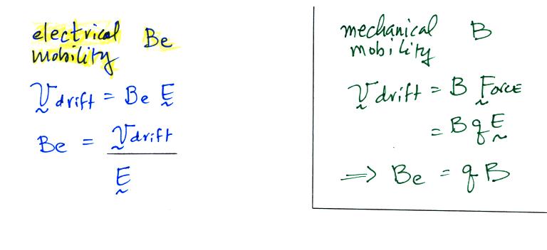
The electrical mobility is a measure of how readily charge carriers will move in an electric field.  The electrical mobility is simply the drift velocity divided by the strength of the electric field.  The relationship between electrical mobility and the mechanical mobility, which is a little more general term, is shown above.


Typical values of Be and drift velocity are shown above.  These drift velocities are much smaller than the random thermal motions of atoms and molecules in air (typically 100s of meters per second). 

Wind motions (typically a few or a few 10s of meters per second) can also potentially transport charge, but for this to occur there must be a gradient is space charge density.  These would be referred to as convection currents.


Here we consider N charge carriers (each with charge q) moving in the same direction and derive an expression for J the current density. 


In general you would need to sum contributions from different charge carriers such as carriers with +q moving in one direction and oppositely charged carriers (-q) moving in the opposite direction.


We've assumed that the number density of positive and negative charge carriers is the same and that the charge carriers carry the same charge and move at the same speed.


Next we derive a continuity equation that relates changes in the space charge density in a volume to net flow of charge into or out of the volume.


Starting at upper left, the charge, Q, contained in the volume is just the volume integral of the volume space charge density.  A positive value for the surface integral of J at upper right would mean net transport of charge out of the volume.  This would reduce the total charge in the volume and dQ/dt would be negative.

We use the divergence theorem to write the surface integral of J as a volume integral of the divergence of J.  Then the two volume integrals are set equal to each other.  The only way the two integrals can be equal for an arbitrary volume is if the integrands themselves are equal.  We end up with the continuity equation highlighted in yellow.  It is then easy to show that under steady state conditions and when J has just a z component, the current density Jz is constant with altitude.


We will only concern ourselves with conduction currents that are linearly proportional to the electric field. 

This is known as Ohm's law and the constant of proportionality is the conductivity.  We can use our newly derived expression for current density together with the definition of electrical mobility to obtain an expression for conductivity. 


Here we've only considered one polarity of charge carriers.  In general there will be both positive and negative charge carriers and the expression for conductivity would have two terms:


We will find that negatively charged small ions generally have slightly higher electrical mobility than postively charged small ions.  Often we will assume that the mobilities and concentrations of positive and negative charge carriers are equal in which case the conductivity would just be 2 N q Be.

A note about conductivity units.


Conductivity has units of 1/(ohms m).  In some older literature you may find this written as mhos/m (mhos is ohms spelled backwards) though Siemens/m are now the officially adopted units.


Resistivity is the reciprocal of conductivity.  Resistivity is not the same as resitance, but it is relatively easy to relate the two.


Resistivities of some common materials are listed below. 

Note how the conductivity of air is a function of air temperature.  A lightning return stroke will heat air to a peak temperature of about 30,000 K for a short time.

Later in the semester we will look at some fast time resolved measurements of lightning electric fields that were being used to try to determine characteristics of the fast time varying currents in lightning strokes.  The measurements were made in a location where propagation between the lightning source and E field antenna was over salt water to preserve as much of the high frequency content of the signals as possible.


Now we go back to something we considered on the first day of the course.  A small portion of the earth's negatively charged surface is shown above.  Negative charge on the ground and positive charge in the atmosphere above creates a downward pointing E field.  We're now in a better position to estimate of how quickly the fair weather current would neutralize the charge on the earth's surface.

We consider the earth's surface to be a perfect conductor.  The vertical E field will depend on the surface charge density, σ.  The current density is just the product of conductivity and electric field.  We end up with a differential equation which we can easily solve for Q, the charge on an area A of the earth's surface.

If we insert reasonable values for εo and λ we obtain

This is the time for the charge on the surface to decrease to 1/e of its original value, not the time needed to neutralize it completely.


An important example problem showing what happens along an air-cloud boundary where there is an abrupt change in conductivity.  


Conductivity inside a cloud is lower than in the air outside a cloud.  This is because the small ions attach to much larger and much less mobile cloud particles (water droplets or ice crystals).  The E field must become stronger inside the cloud so that the current density (the produce of conductivity and electric field) stays the same inside as outside the cloud.  We'll see that layers of charge build up on the top and bottom surfaces of the cloud. 

We'll try to estimate how much charge is necessary


We don't really know Ez.  Jz on the other hand is constant with altitude and we assume we know how conductivity changes as you move across the cloud-air boundary.

We can integrate this equation

So we conclude a layer of positive charge builds up on the top edge of the cloud.  In a similar kind of way you could show that a layer of negative charge would build up on the bottom edge of the cloud.


The effect of these two layers of cloud is to intensify the field inside the cloud.  The product of higher field times lower conductivity inside the cloud is able to keep the current density equal to the current density outside the cloud.

Screening layers that form along the edges of a thunderstorm effectively mask the main charge centers inside the cloud.


One of the consequences of this is that it makes it difficult to use measurements of E field at the ground to estimate how much charge builds up inside the cloud.