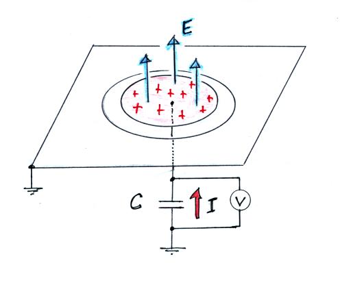
An electric field antenna that is
not flush with the ground surface will distort the surrounding electric
field. This is an appropriate point to review a problem worked in
most undergraduate electricity and magnetism courses (the notes that
follow are based on a class handout prepared by Dr. E. Philip Krider).
Conducting Sphere in a
Uniform Electric Field
Notes on the distortion of an initially uniform
electric field Eo by the presence of an uncharged conducting
sphere. The sphere distorts the field such that the field lines
are everywhere normal to the surface of the conductor. Choosing
the origin of our coordinate system at the center of the sphere,
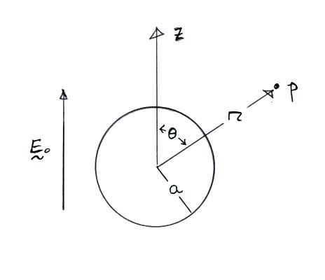
Spherical polar coordinates are
used, there is azimuthal symmetry, so the potential and the electric
field depend on r and θ
only. We can proceed to solve
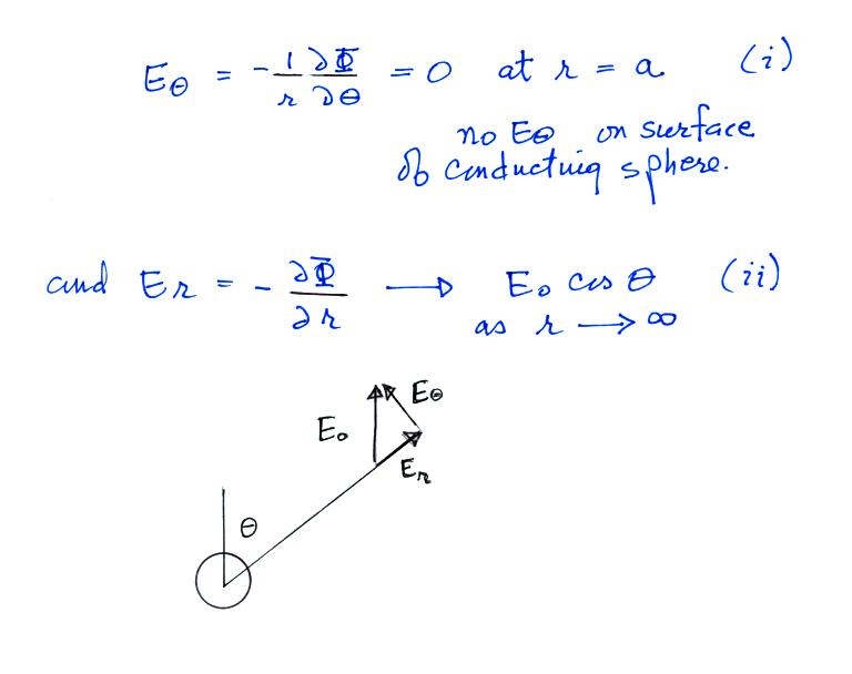
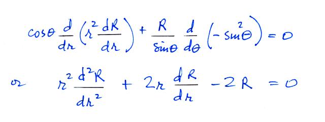
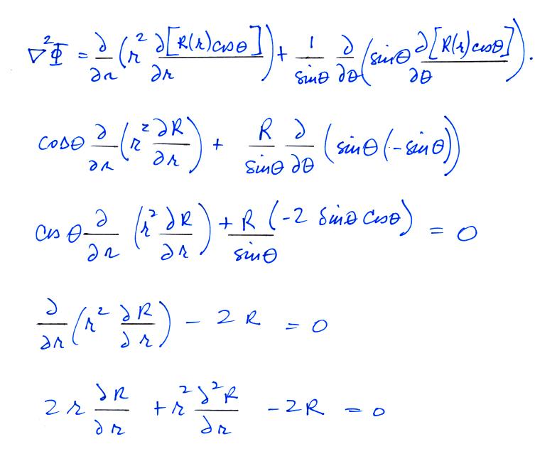
Laplace's equation for the potential, Φ, subject to the boundary
conditions that
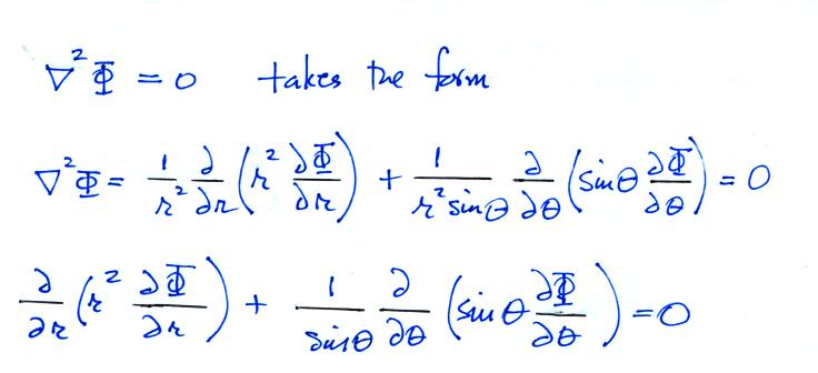
In the spherical coordinate
system
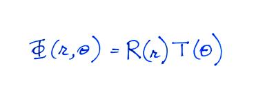
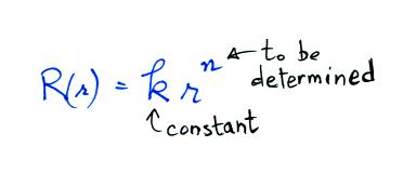
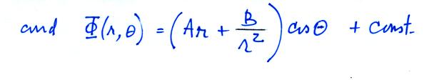
Assuming the variables are separable, we try a general
solution of the form:
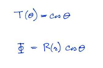
Just looking at the boundary condition (Eqn. (ii)), we simply try
a T(θ) function of the form
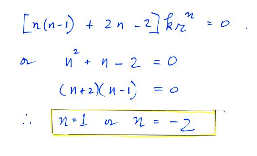
Now, inserting this into our original differential equation, we
find
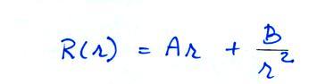
and
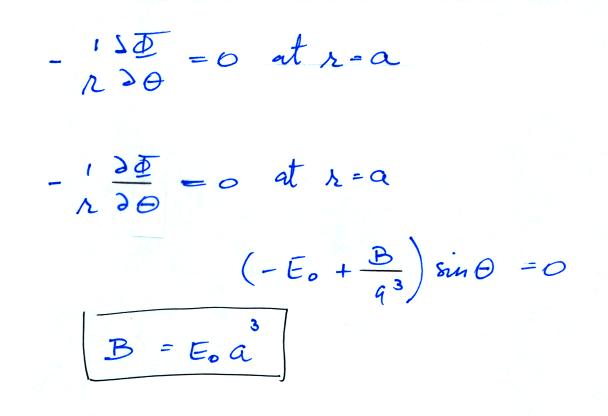
Where A and B must be determined
from the boundary conditions.
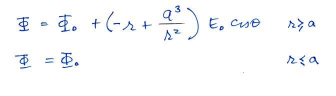
Now,
applying boundary condition (ii) as
r goes to infinity
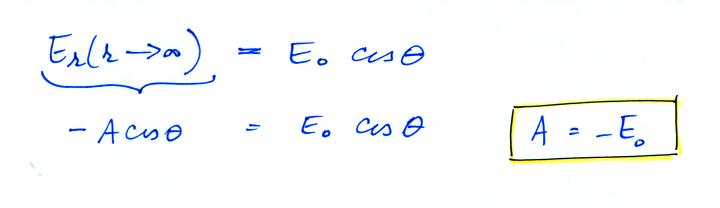
since
and our potential function is now
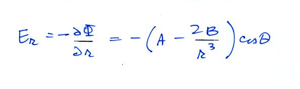
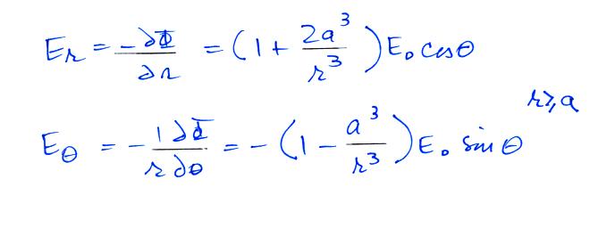
with this Φ our electric field components are:
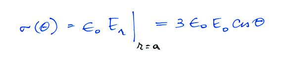
and the surface charge density is
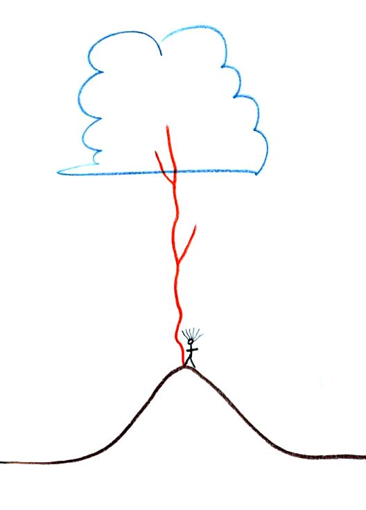
Note: The presence of the sphere increases the value of the ambient
field at the top and bottom surface of the sphere by a factor of 3.
This figure gives you a rough idea
of how the field is changed in the vicinity of the sphere. E
field lines must intersect the sphere perpendicularly. The field is
enhanced (amplified) by a factor of three at the top and bottom of the
sphere.
Enhancement
of
fields by conducting objects is an important concern. In some
cases (we'll look at an example or two later) the enhanced field is
strong enough to initiate or trigger a lightning discharge.
The following handout gives a rough, back-of-the-envelope kind of
estimate of the factor of enhancement.
This might require a little
explanation.
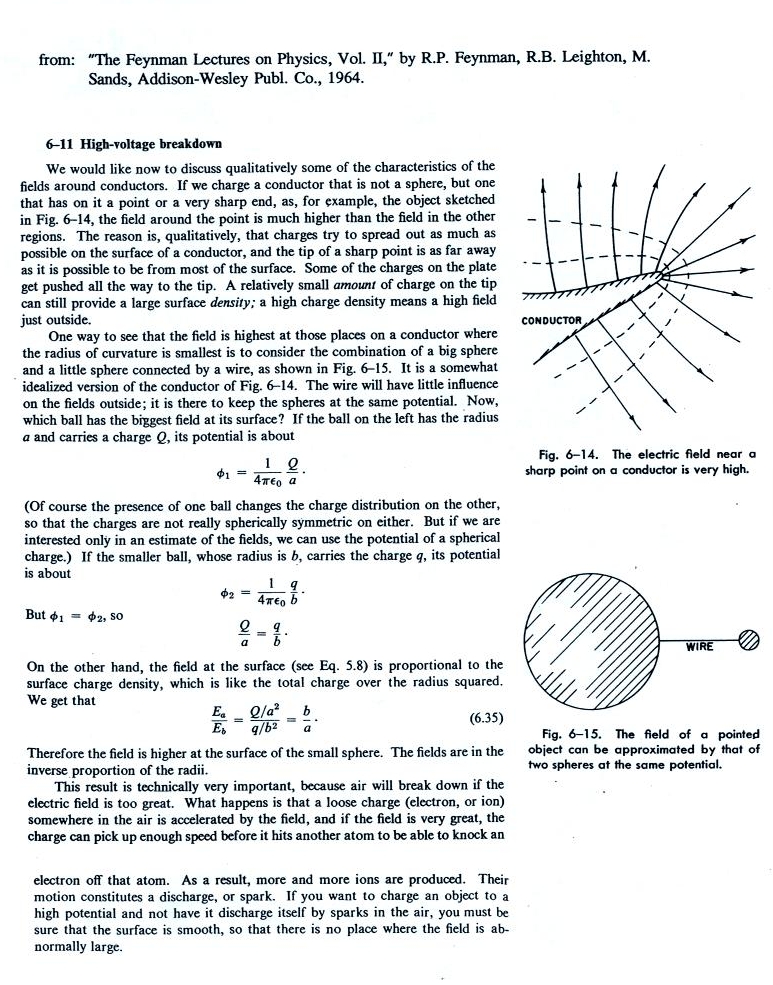
First you write down the potential
at the surface of two conducting spheres of radius a and b, carrying
charges Q and
q (really just the potential a distance a or b from a point charge Q or
q)
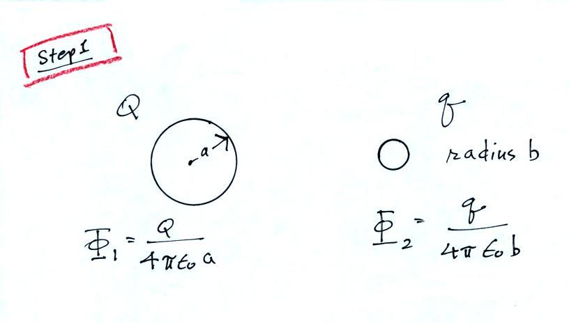
Then you connect the two spheres
with a wire which forces the two
potentials to be equal (this would of course cause the charge to
rearrange themselves and turn this into a much more complex problem,
but we will ignore that).
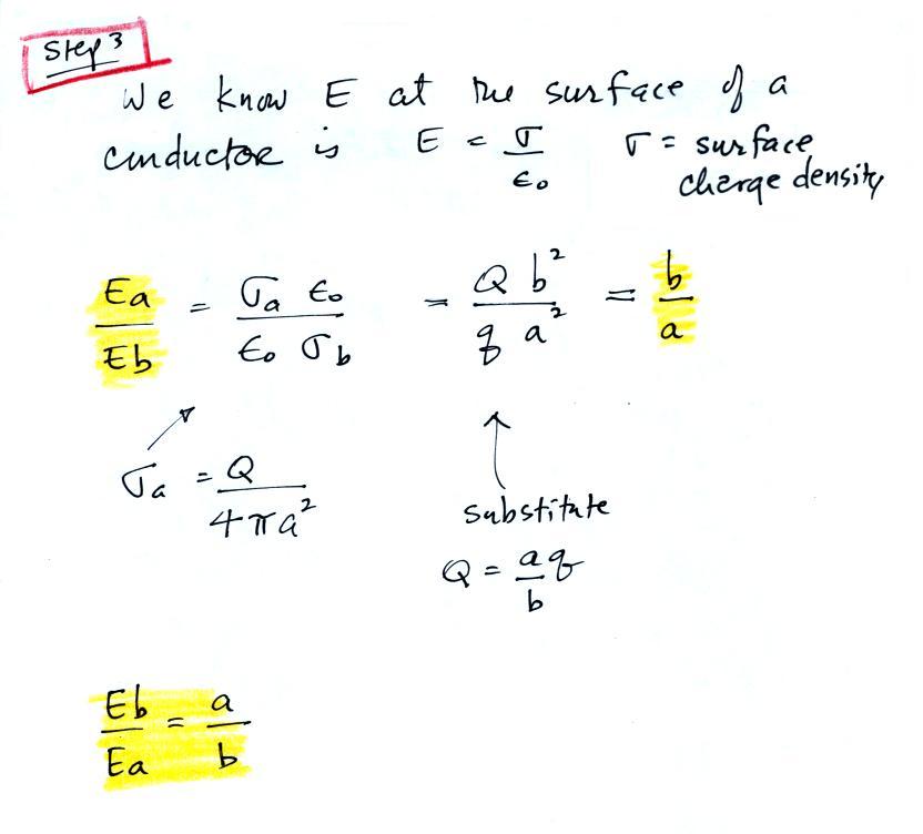
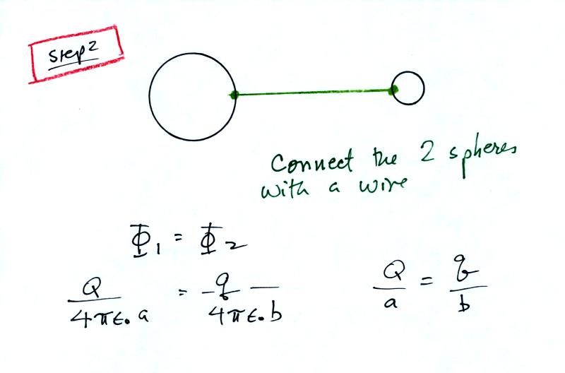
Finally we write down expressions
for the relative strengths of the
electric fields at the surfaces of the two spheres. We see that
the field at the surface of the smaller sphere is a/b times larger than
the field at the surface of the bigger sphere.
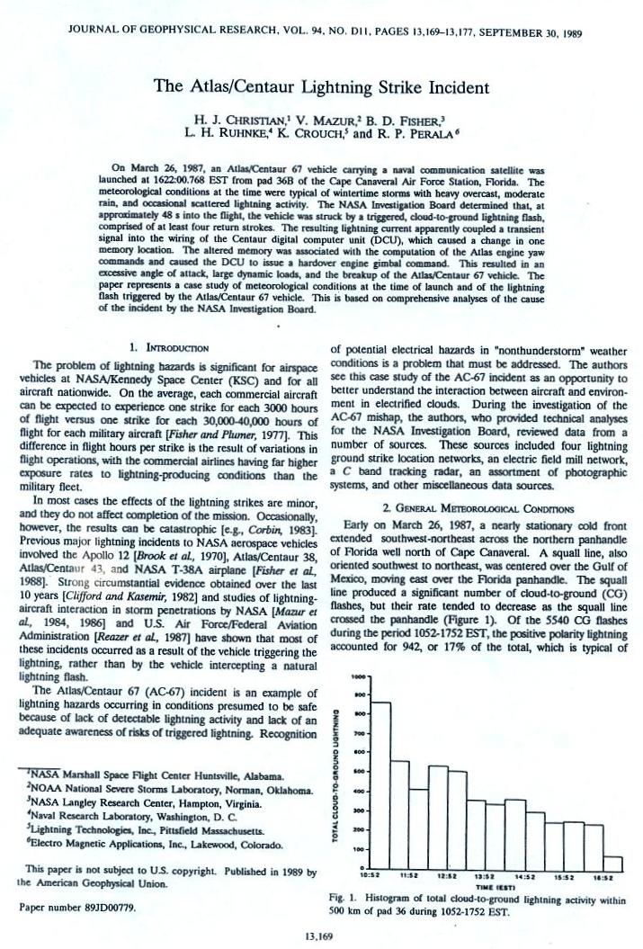
Here is a
real example of field enhancement that lead to triggering of a
lightning strike and subsequent loss of a launch vehicle (you'll find
the entire article here)
In this case the rocket body together with the exhaust plume created a
long pointed conducting object. Enhanced fields at the top and
bottom triggered lightning.
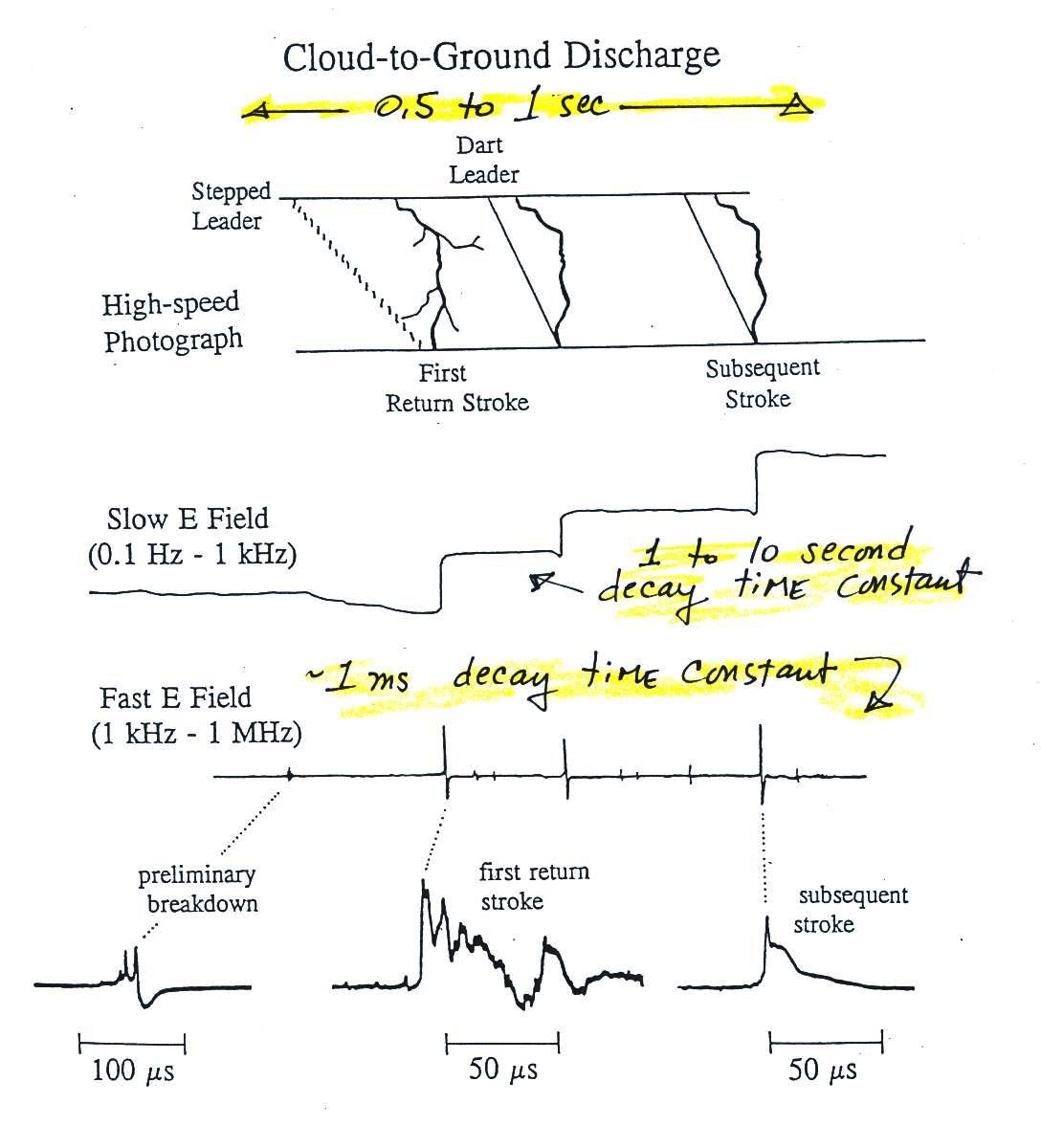
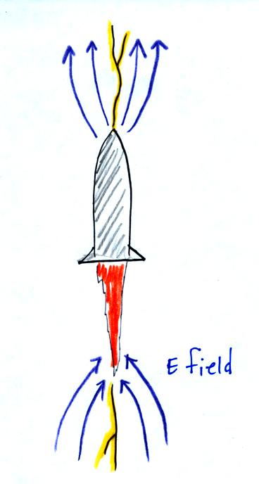
Lighning is sometimes triggered at the tops of tall mountains
Note the direction of the branching. This indicates that
this discharge began with a leader process that traveled upward from
the mountain. Most cloud to ground lightning discharges begin
with a leader that propagates from the cloud downward toward the
ground. We will of course look at the events that occur during
lightning discharges in a lot more detail later in the
semester.