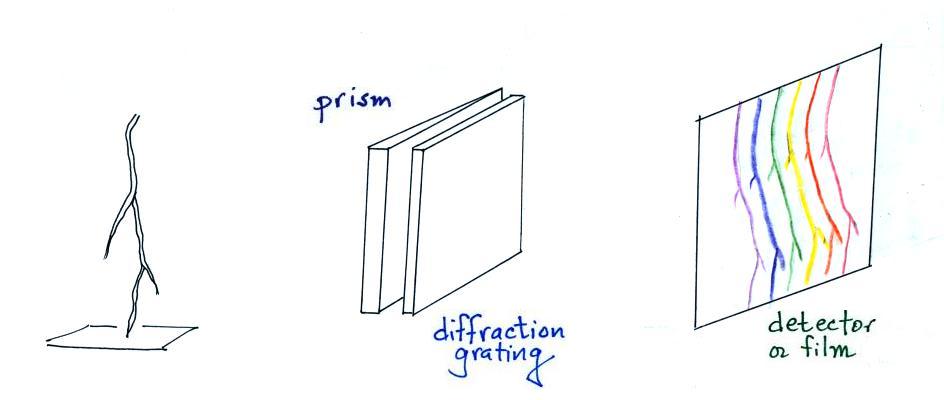
Here's a illustration of the
slitless spectrograph technique, mentioned briefly in Lecture 24, that
can be used for lightning. Light from a lightning channel
passes through both a prism and a diffraction
grating and is imaged on film (or a detector of some kind). An
entrance slit is not needed because the lightning source is already a
narrow channel. The spectrum that you would obtain in this case
would be an integration of all the emissions that occurred during the
whole discharge.
To obtain a time resolved spectrum we need to add a horizontal slit to isolate just a segment of the lightning channel and then cause the film to move perpendicularly.
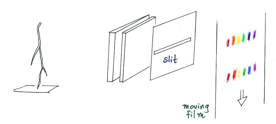
To obtain a time resolved spectrum we need to add a horizontal slit to isolate just a segment of the lightning channel and then cause the film to move perpendicularly.
The film is shown moving downward
in this picture (and sorry that the perspective isn't quite
right). Spectra from two separate return strokes, perhaps, have
been recorded on the film.
Here are actual implimations that provide moderate and very fast time resolution (from E.P. Krider, "Lightning Spectrosocpy," Nuclear Instruments and Methods, 110, 411-419, 1973).
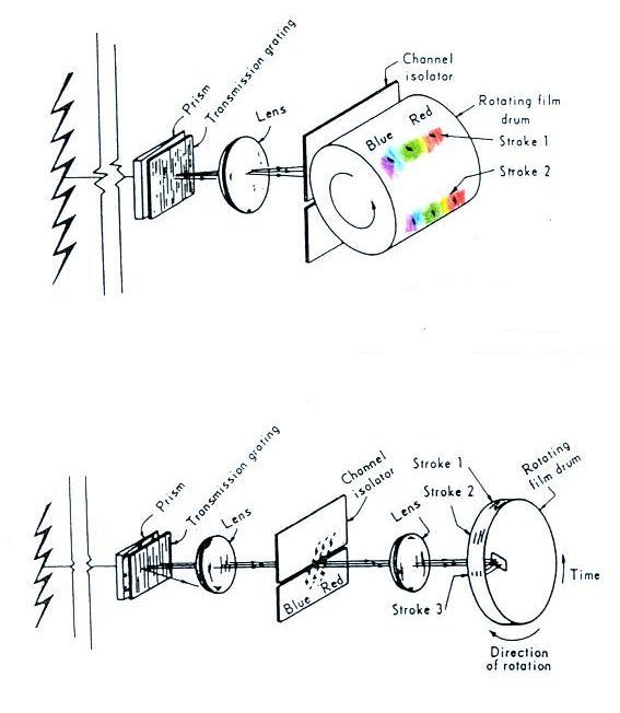
The rotating drum in the lower figure provides the fastest time resolution. Rapidly rotating drums in streaking cameras are also used in photographic measurements of return stroke velocity.
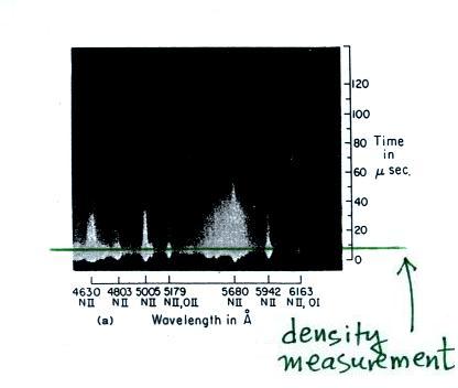
The next figure shows an actual example of a very fast time resolved spectrum from a return stroke.
Here is an example of a "digitized" spectrum. Film's response to light is nonlinear, so the film must be calibrated. Film also reacts different to short bright impulses of light than it does to longer duration low amplitude light signals. So that effect must also be considered.
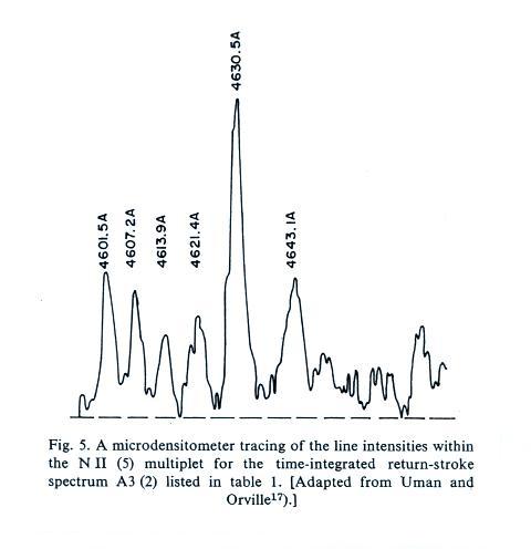
Six emission lines in the NII(5) multiplet spectrum above have been identified. I am not familiar enough with spectroscopy and quantum mechanics to be able to say for sure what precise states and transitions cause these features
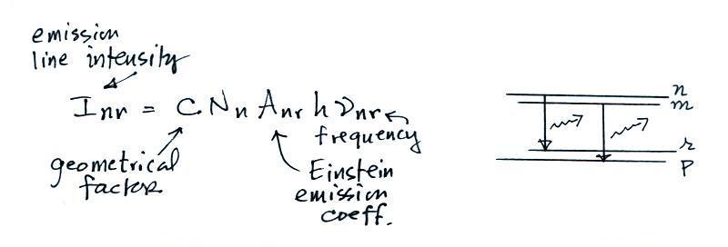
The intensity of the emission produced by transitions from energy level n to r is shown above.
Now we will look at the ratio of measured intensities from two different transitions: n to r and m to p
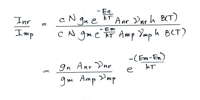
It is these transition intensities that can be measured on the
fast time resolved lightning spectra. Note that many of the
parameters cancel. This is fortunate because some of them (such
as the geometric factor) might be difficult to determine. Solving
for
temperature yields
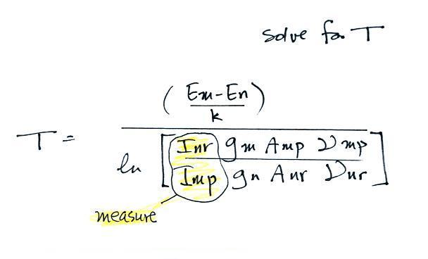
Often what is done is that several determinations of temperature
are made using different combinations of lines in the multiplet group
and an average is computed. In the case of the NII(5) multiplet 5
ratios could be computed: 4630/4601, 4630/4607, 4630/4613, 4630/4621,
and 4630/4643.
The next several figures shown some of the results of these spectroscopic measurements and analyses.
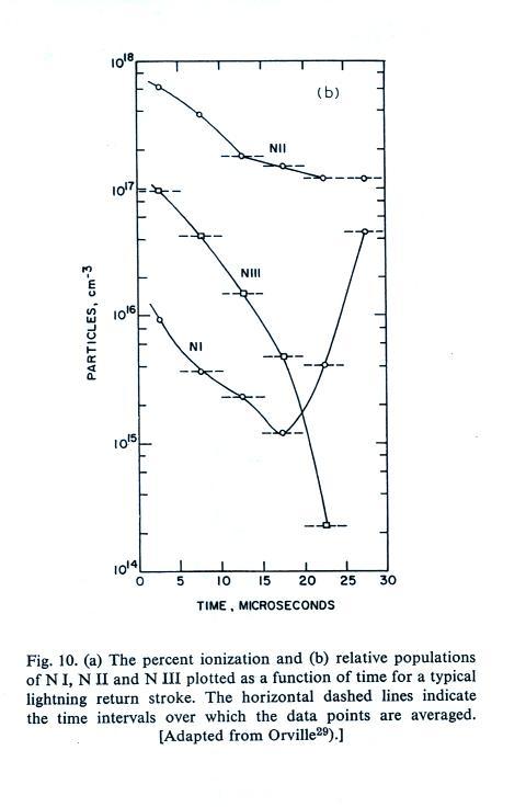
Concentrations of NIII (doubly ionized atomic nitrogen), NII (singly ionized atomic nitrogen), and NI (neutral atomic nitrogen) early in a return stroke discharge. NII is initially the most abundant species and is used in spectroscopic determinations of peak temperature in the return stroke channel.
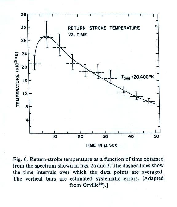
Estimate of peak return stroke channel temperature. The
value approaches 30,000 K which is approximately 5 times hotter than
the surface of the sun (6000 K).
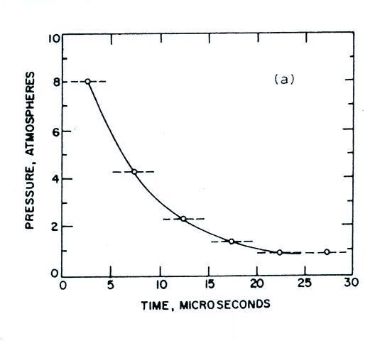
Here are estimates of channel pressure. This requires a
measurement of temperature and probably density (including electron
density from the ionized air molecules).
Thunder
Early in a return stroke, pressure in the channel is several times (maybe a few 10s of times) atmospheric pressure. The lightning channel expands rapidly outward initially as a shock wave. Much of the energy in a lightning stroke is dissipated during the formation and outward growth of the shock wave. The shockwave expands outward a few meters in 10s of microseconds and quickly decays into the sound wave that we eventually hear as thunder.
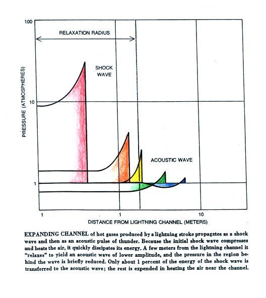
This figure (this and the next two figures are from an article on
Thunder by A.A. Few that appeared in "The Physics of Everyday
Phenomena", Readings from Scientific American, W.H. Freeman & Co,
San Francisco, 1979) shows the transition from shock wave to sound
wave. The size of the channel when this occurs (a few meters) is
referred to as
the relaxation radius. Channel tortuosity features
that are smaller than the relaxation radius are swallowed up by the
shock wave and don't really affect properties
of the thunder such as frequency.
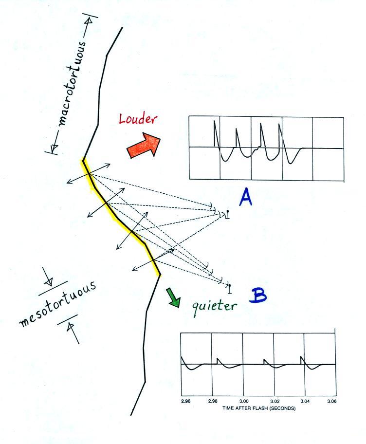
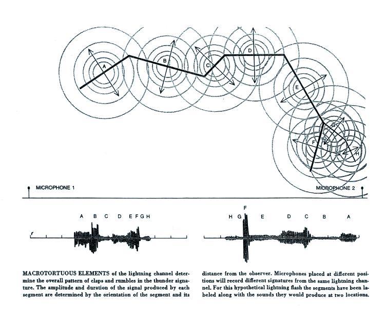
Lightning channels consist first of mesotortuous segments that are 5 to a few 10s of meters long. Several of these positioned end-to-end and oriented in about the same direction form a macrotortuous segment. The variation of sounds that are heard during thunder are determined primarily by your orientation relative to the mesotortuous elements. Sounds emitted in a direction that perpendicular to the channel are louder than sounds emitted more nearly parallel to the channel.
Microphone A is located more nearly perpendicularly to the 4 mesotortuous segments highlighted in the figure. Four relatively loud sound pulses arrive in quick succession at microphone A and form a clap of thunder. Microphone B is positioned more nearly end. Weaker impulses arrive at the second microphone over a longer period of time and produce more of a rumble.
Another, more realistic, illustration of how the pattern of sounds in thunder and the duration of the thunder depend on your location and the geometry of the lightning channel.
It is generally not possible to separate the sounds of the separate return strokes in a thunder record (either by ear or on thunder recordings). A sound that resembles "tearing cloth" has often been reported a split second before the loud clap of thunder from a close lightning strike. When I mention this in the lecture version of this class, most students agree that they have heard something like this. The cause of that sound is not known.
Thunder duration is examined is a bit more detail in the next figure (from: M.A. Uman, The Lightning Discharge, Ch. 15, Academic Press, Orlando, 1987).
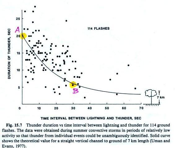
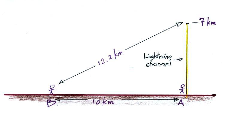
The points on the graph shows actual measurements of thunder duration from discharges at different distances from the observer. The solid line is a calculation of thunder duration from a vertical lightning channel 7 km tall. Points A and B highlighted above refer to the calculations below.
Person A in the figure above will hear the thunder coming from the
bottom of the channel instantaneously. Sound travels about 340
m/sec in 20 C air (1 km in 3 seconds, 1 mile in approximately 5
seconds), so the sound from the top of the channel will arrive about 21
seconds later. That's a duration of 21 seconds.
The observer at Point B will hear the thunder from the bottom of the channel 30 seconds after the lightning strike. The bottom of the channel is 10 km away from the observer. The top of the channel is 12.2 km away, so thunder coming from the top of the channel will arrive about 6.6 seconds later than the sound coming from the bottom of the channel (3 seconds/km x 2.2 km). The thunder only lasts for about 6.5 seconds at Point B.
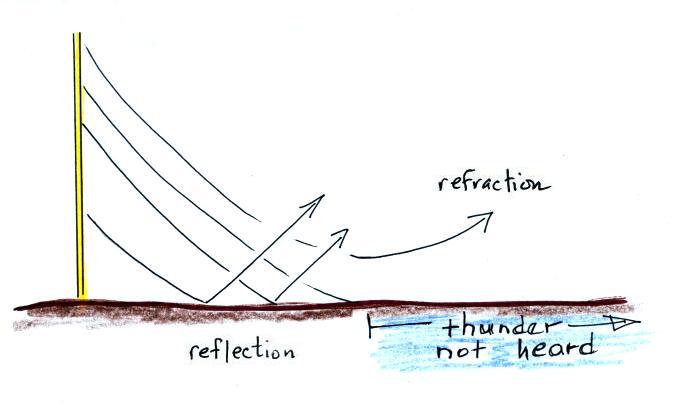
Wind can affect the sound of thunder and refraction can mean there is a distance beyond which thunder is not heard
Here are actual implimations that provide moderate and very fast time resolution (from E.P. Krider, "Lightning Spectrosocpy," Nuclear Instruments and Methods, 110, 411-419, 1973).
The rotating drum in the lower figure provides the fastest time resolution. Rapidly rotating drums in streaking cameras are also used in photographic measurements of return stroke velocity.
The next figure shows an actual example of a very fast time resolved spectrum from a return stroke.
Several emission features are
identified on this spectrum early in the return stroke discharge (NII
is a singly ionized nitrogen atom). Now what is usually done next
is to scan across the film image using a densitometer at say perhaps
the level of the green line (i.e. at a time about 10 microseconds after
the beginning of the return stroke).
Here is an example of a "digitized" spectrum. Film's response to light is nonlinear, so the film must be calibrated. Film also reacts different to short bright impulses of light than it does to longer duration low amplitude light signals. So that effect must also be considered.
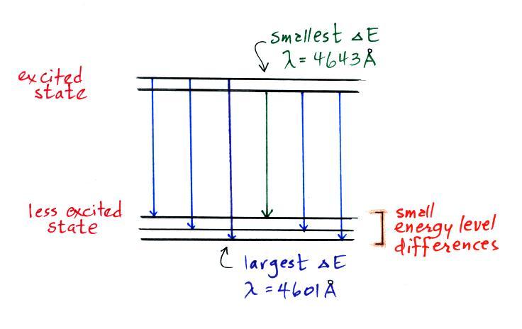
Six emission lines in the NII(5) multiplet spectrum above have been identified. I am not familiar enough with spectroscopy and quantum mechanics to be able to say for sure what precise states and transitions cause these features
but I'm guessing it looks something
like shown here. Transitions from 2 slightly different energy
levels from an excited state to 1 of 3 levels at a lower energy state
could produce emissions of 6 slightly different wavelengths.
In any event it is the relative amplitudes of lines in a multiplet group that can be used to estimate lightning channel temperature. The procedure is described below. Our goal is not understand all the steps but rather to get a flavor for the procedure or method.
The first assumption made is that the number of atoms in a particular energy level can be described using a Maxwell-Boltzmann distribution
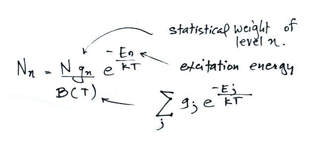
Nn is the number of atoms in energy level n, N is the total number of atoms.
In any event it is the relative amplitudes of lines in a multiplet group that can be used to estimate lightning channel temperature. The procedure is described below. Our goal is not understand all the steps but rather to get a flavor for the procedure or method.
The first assumption made is that the number of atoms in a particular energy level can be described using a Maxwell-Boltzmann distribution
Nn is the number of atoms in energy level n, N is the total number of atoms.
The intensity of the emission produced by transitions from energy level n to r is shown above.
Now we will look at the ratio of measured intensities from two different transitions: n to r and m to p
The next several figures shown some of the results of these spectroscopic measurements and analyses.
Concentrations of NIII (doubly ionized atomic nitrogen), NII (singly ionized atomic nitrogen), and NI (neutral atomic nitrogen) early in a return stroke discharge. NII is initially the most abundant species and is used in spectroscopic determinations of peak temperature in the return stroke channel.
Thunder
Early in a return stroke, pressure in the channel is several times (maybe a few 10s of times) atmospheric pressure. The lightning channel expands rapidly outward initially as a shock wave. Much of the energy in a lightning stroke is dissipated during the formation and outward growth of the shock wave. The shockwave expands outward a few meters in 10s of microseconds and quickly decays into the sound wave that we eventually hear as thunder.
Lightning channels consist first of mesotortuous segments that are 5 to a few 10s of meters long. Several of these positioned end-to-end and oriented in about the same direction form a macrotortuous segment. The variation of sounds that are heard during thunder are determined primarily by your orientation relative to the mesotortuous elements. Sounds emitted in a direction that perpendicular to the channel are louder than sounds emitted more nearly parallel to the channel.
Microphone A is located more nearly perpendicularly to the 4 mesotortuous segments highlighted in the figure. Four relatively loud sound pulses arrive in quick succession at microphone A and form a clap of thunder. Microphone B is positioned more nearly end. Weaker impulses arrive at the second microphone over a longer period of time and produce more of a rumble.
Another, more realistic, illustration of how the pattern of sounds in thunder and the duration of the thunder depend on your location and the geometry of the lightning channel.
It is generally not possible to separate the sounds of the separate return strokes in a thunder record (either by ear or on thunder recordings). A sound that resembles "tearing cloth" has often been reported a split second before the loud clap of thunder from a close lightning strike. When I mention this in the lecture version of this class, most students agree that they have heard something like this. The cause of that sound is not known.
Thunder duration is examined is a bit more detail in the next figure (from: M.A. Uman, The Lightning Discharge, Ch. 15, Academic Press, Orlando, 1987).
The points on the graph shows actual measurements of thunder duration from discharges at different distances from the observer. The solid line is a calculation of thunder duration from a vertical lightning channel 7 km tall. Points A and B highlighted above refer to the calculations below.
The observer at Point B will hear the thunder from the bottom of the channel 30 seconds after the lightning strike. The bottom of the channel is 10 km away from the observer. The top of the channel is 12.2 km away, so thunder coming from the top of the channel will arrive about 6.6 seconds later than the sound coming from the bottom of the channel (3 seconds/km x 2.2 km). The thunder only lasts for about 6.5 seconds at Point B.
Wind can affect the sound of thunder and refraction can mean there is a distance beyond which thunder is not heard
 |
 |
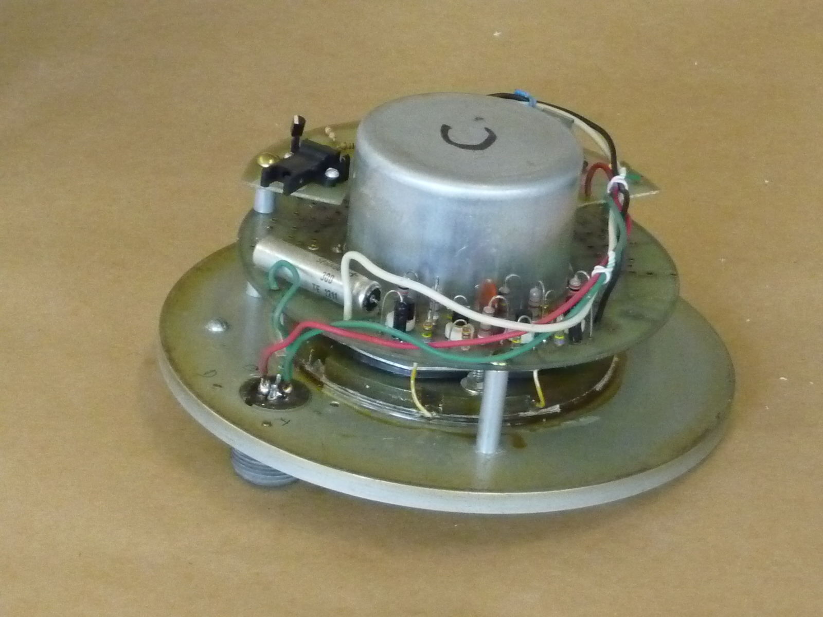 |
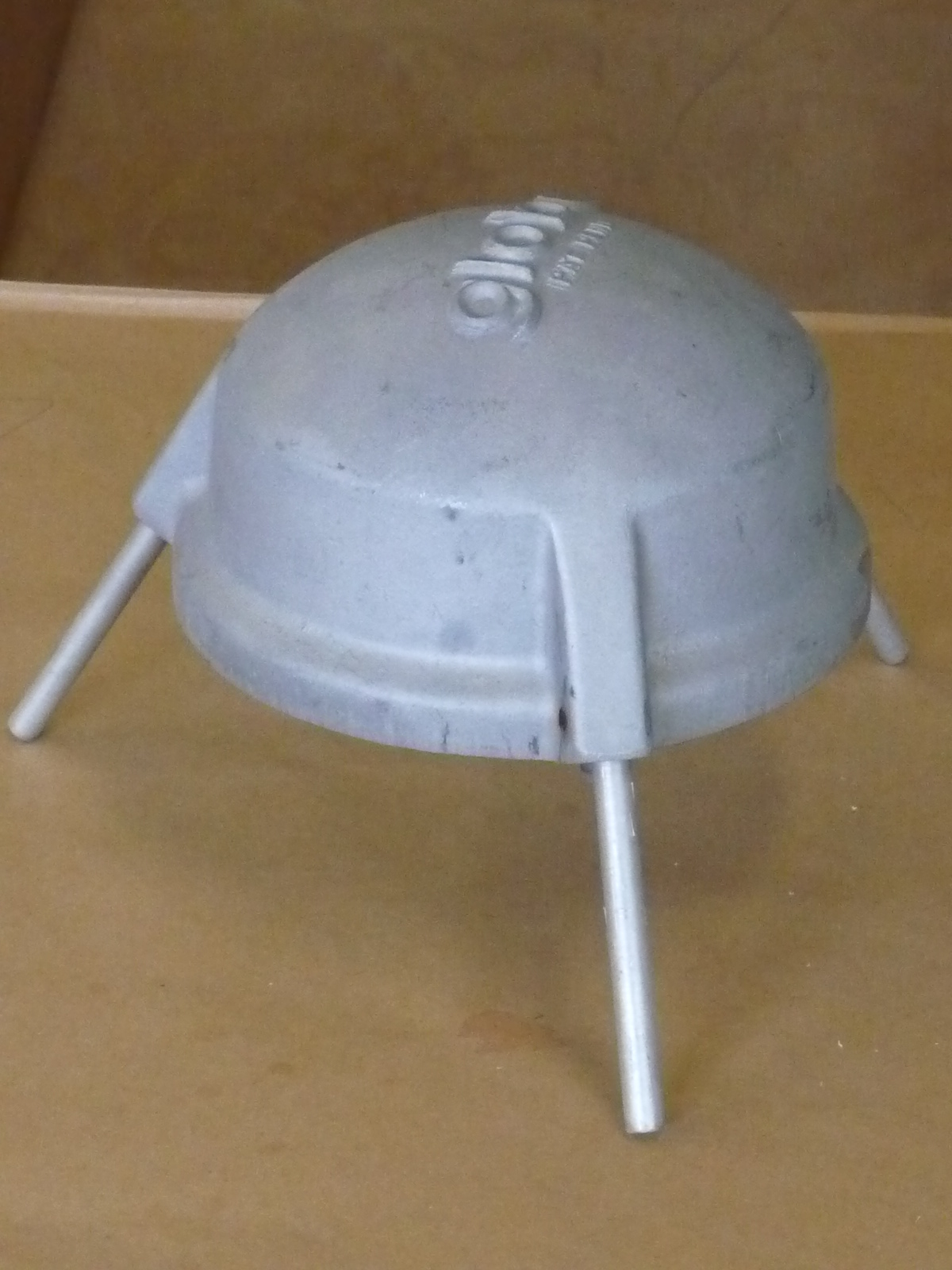
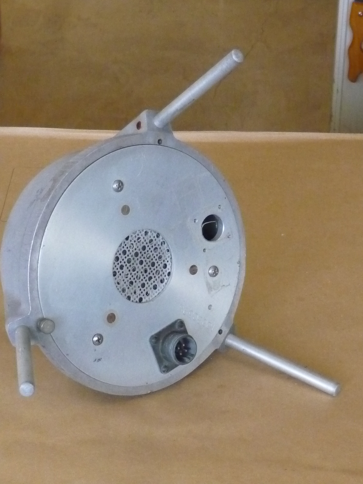
These are pictures of a microphone
that has been used to make thunder measurements in the infrasonic to
low audio frequency range (a Globe Model 100-B Capacitor
Microphone). The microphone consists of a flexible diaphragm and
a metal back plate which act as plates of a capacitor. The
microphone is normally set up right as shown in the left most figure
(the metal housing is sometimes covered with a "rubberized hair" wind
screen (similar to the "rat's hair" used as a packing material).
The microphone has been turned on its side, in the center picture, to
shown the opening that exposes the microphone to the pressure changes
caused by thunder. The right most picture shows the microphone
electronics.
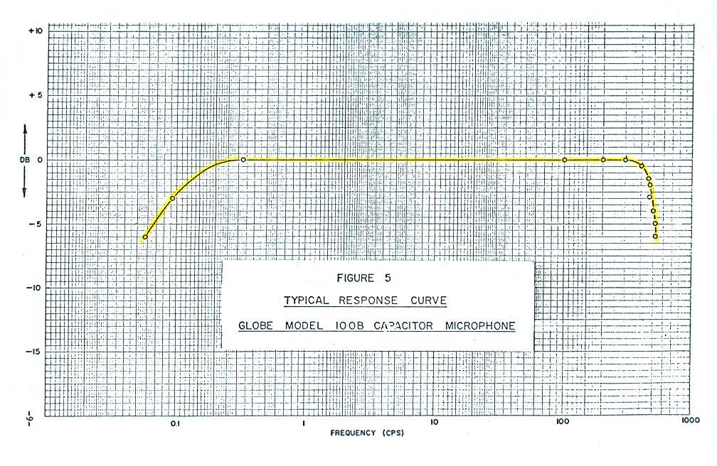
Calibrated response of the Globe capacitor microphone. The microphone response is flat from about 0.5 Hz to about 300 Hz.
Calibrated response of the Globe capacitor microphone. The microphone response is flat from about 0.5 Hz to about 300 Hz.
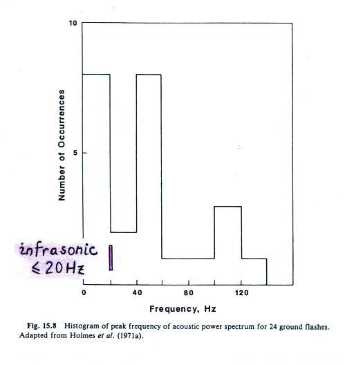
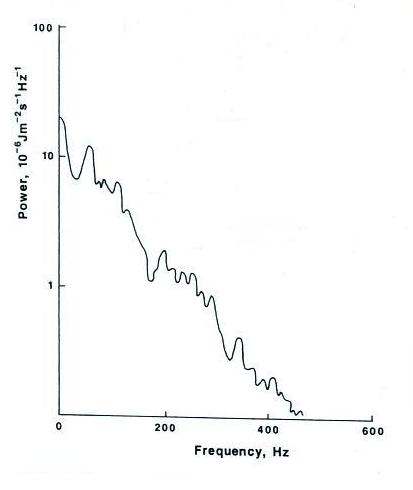
Here are three plots of the
measured thunder frequency spectra
This first plot is actually a
distribution of peak values in sound spectra. Interestingly a
portion of the distribution is below 20 Hz and is inaudible; this is infrasound.
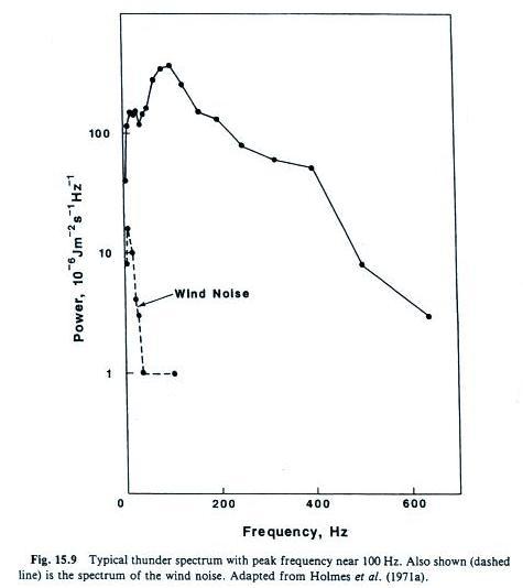
This is the spectrum from a single discharge. The peak in the spectrum is near 100 Hz.
This is the spectrum from a single discharge. The peak in the spectrum is near 100 Hz.
An example of a sound spectrum
(lower right corner) that actually peaks in the infrasound.
Up to this point we have explained thunder as being due to the explosive expansion of a hot lightning channel. This may not be the cause of all of the emissions at infrasonic frequencies. Some researchers have suggested that a sudden change in the cloud electrostatic field caused by a lightning discharge might be the cause of the very low frequency infrasonic emissions.
Up to this point we have explained thunder as being due to the explosive expansion of a hot lightning channel. This may not be the cause of all of the emissions at infrasonic frequencies. Some researchers have suggested that a sudden change in the cloud electrostatic field caused by a lightning discharge might be the cause of the very low frequency infrasonic emissions.