Lecture 25 - Ground based optical observations of lightning

In this lecture we'll look at ground-based measurements of the optical emissions produced by lightning.

Lightning is a pretty bright light source and a simple photodiode can, in most cases, be used to detect lightning optical signals.

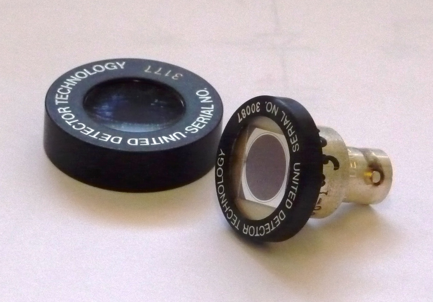
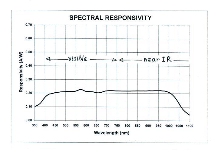
A typical silicon photodiode (at right, a PIN 10 DF diode manufactured by United Detector Technology). This particular photodiode has an active (sensing) area of 1.0 cm². It can also be fitted with a blue filter (shown at left in the photograph above) which results in fairly flat wavelength response across the visible and part of the near IR portions of the spectrum (a representative spectral response curve is shown below).

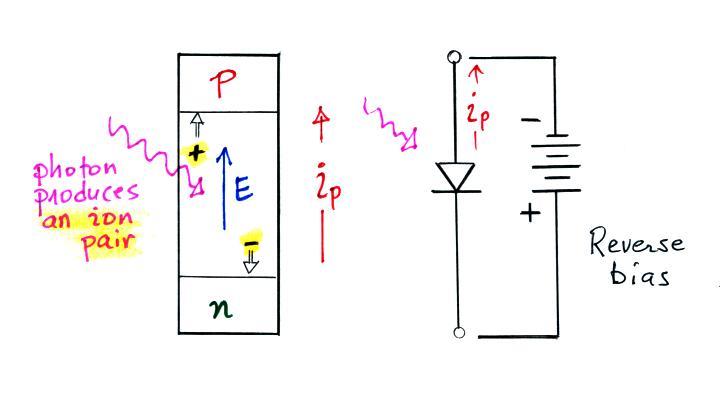
Photodiodes like this are often operated in the photoconductive mode (the diode produces a current that is proportional to the intensity of the incident light signal) and are back biased. This provides fast time response. This is explained further in the next few figures.

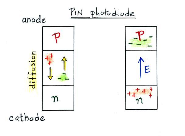
A PIN photodiode (and this is my very incomplete understanding of them) consists of a "p-doped" region, a middle intrinsic (undoped) region, and an "n-doped" region. The term "doping" means impurities have been added to a semiconductor material such as silicon. An n-doping material (such as phosphorus) effectively adds negative polarity charge carriers, the p-doping material (boron or aluminum) positive charge carriers. Charge diffuses from the doped regions across the intrinsic region in the middle. Movement of the charge carriers creates an electric field which, once it grows to sufficient strength, limits further diffusion and further charge buildup.

Photons which strike the intrinsic region of the photodiode produce photo ions which then move under the influence of the E field. Back biasing the photodiode increases the size of the intrinsic region and accelerates movement of the photo ions.

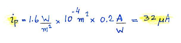
We'll do a quick calculation to estimate a typical lightning photo current, i_p. We'll assume a sensing area of 1.0 cm², a responsivity of 0.2 A/W and an incident irradiance of 1.6 W/m² (more about this value later in the lecture notes).

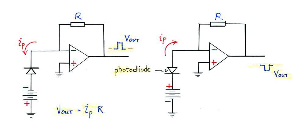
A current this small is readily converted to a measureable voltage using one of the basic op-amp (operational amplifier) circuits below.

The two circuits are identical except for the orientation of the photodiode and the polarity of the biasing voltage. The orientation in the top figure gives a positive-going output signal. The bottom circuit produces a negative polarity output. A feedback resistance of 50 kΩ and a photo current of 32 μA would produce an output voltage of 1.6 volts.

Now we'll look at some actual data. Most of the results will come from "The Optical and Radiation Field Signatures Produced by Lightning Return Strokes," C. Guo and E.P. Krider, J. Geophys. Res., 87, 8913-8922, 1982) which used a fairly straightforward sensor design.

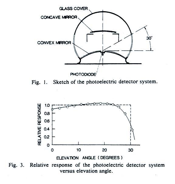
In this case a silicon photodiode was used together with a few optical components to produce a system with 360 degree azimuthal response and fairly flat angular response between 0 and about 25 degrees elevation angle. This field of view would be sufficient to see the entire lightning channel between the ground and cloud base unless the lightning was close to the observing location.

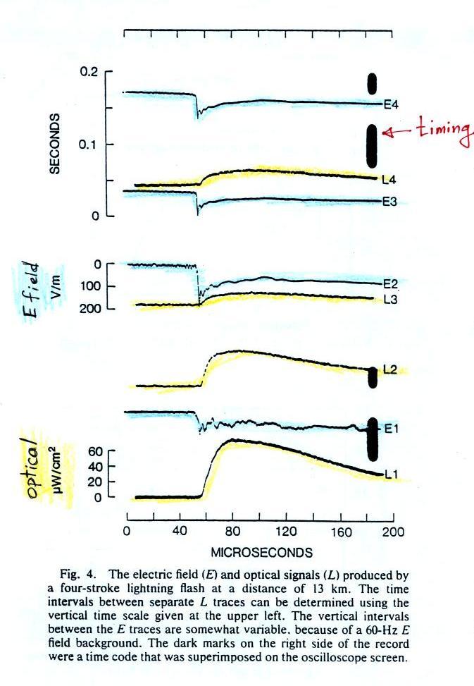
Examples of recorded fast electric fields (E, shaded blue) and associated optical signals (O, highlighted in yellow). This was a four stroke cloud-to-ground discharge that occurred at 13 km range. The first return stroke is shown at the bottom of the figure. The first 50 μs or so of the record is the stepped leader. This is followed by an abrupt rise to peak. Notice that the E field signal is still increasing in ampltitude at the end of the record. This indicates some of the electrostatic field component is present which is typical of a return stroke field recorded at a range of about 10 km. These waveforms were photographed on moving film. The dark black timing marks were from an LED that would flash on and off to code the absolute time onto the film.

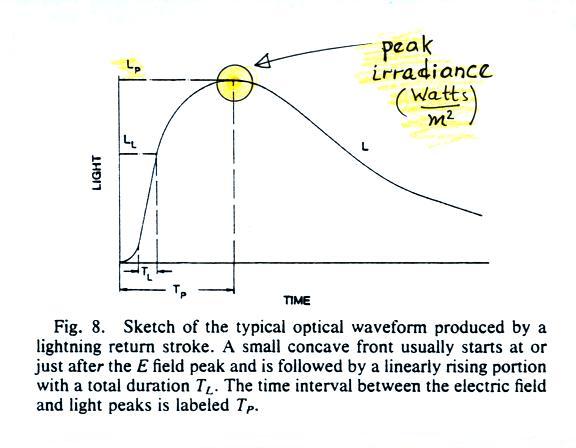
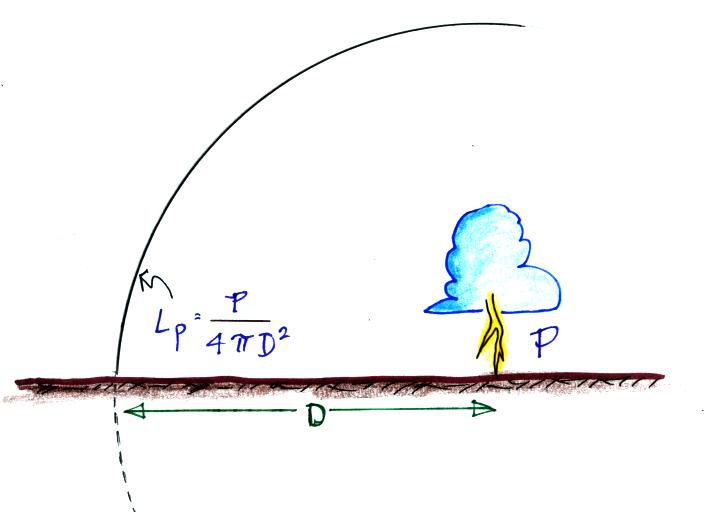
A typical return stroke optical signal. We can use a measurement of the peak optical signal amplitude (in volts) to determine the peak irradiance, L_p (in W/m²). Then if the range to the discharge is known we can estimate the peak optical power output, P (in Watts) from the return stroke.

We treat the lightning discharge as a point source and assume the optical power output during the strike will expand evenly outward in a sphere. We measure the peak irradiance, L_p, a distance D from the source (W/m² on the surface of the expanding sphere). So to estimate P we simply multiply the measured values of L_p by the area of the sphere.

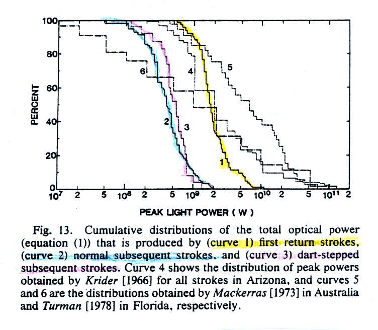
Here's a cumulative distribution of peak optical power estimates. 50% of 1st return strokes have a peak optical power output of about 2 x 10⁹ Watts or more. Peak power emitted by subsequent strokes is almost a factor of 10 less.

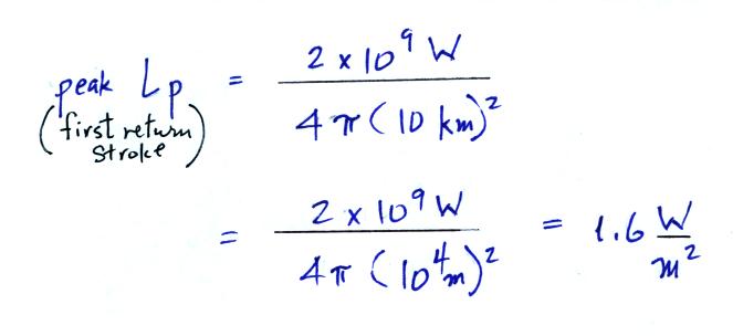
Peak irradiance from a return stroke at 10 km range would be about

You may remember this is the value used to compute an expected photodiode output current.

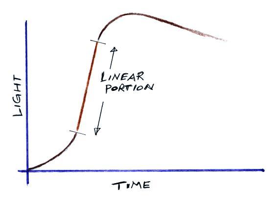
Next we will consider the linear portion of the rising front on a lightning optical waveform.

We will assume that this is produced by the geometric growth of the return stroke channel as it propagates from the ground up toward the bottom of the cloud (the signal amplitude grows as the channel gets taller). We'll also assume the channel is straight and vertical and that the return stroke velocity is constant.

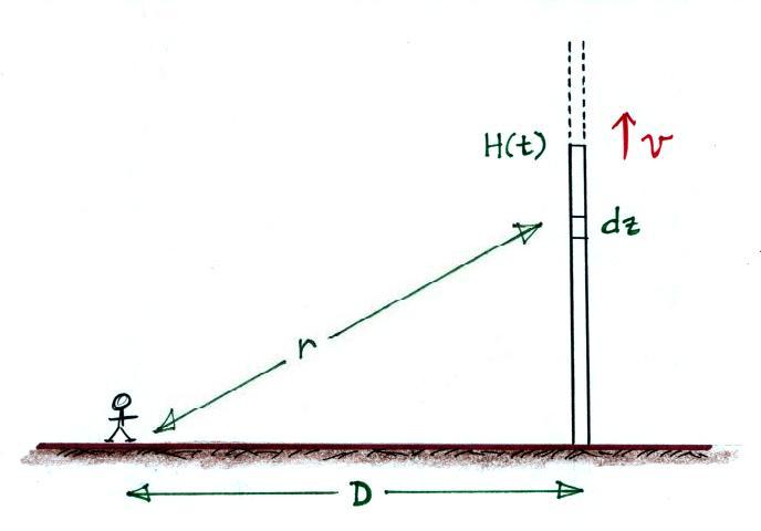
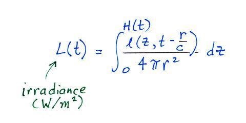
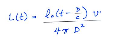
Optical emissions from the length of the channel between the ground and H(t) determine the amplitude of the signal observed at distance D at time t.

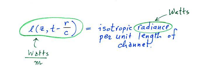
The equation is pretty general at this point, we allow l(z,t) to vary with z and t.

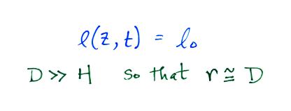
We'll make a couple of simplifying assumptions

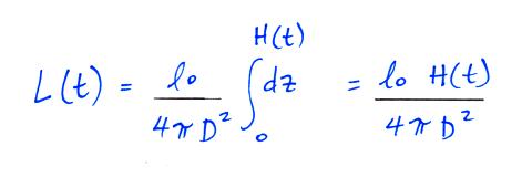
Then the integral becomes

we'll replace H(t) with a time multiplied by velocity term

Here you can clearly see that L(t), measured at distance D would increase linearly with time.
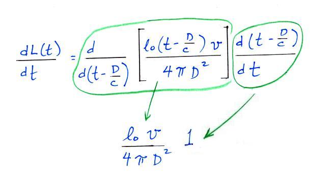
Next we differentiate this expression

dL(t)/dt is just the slope of the linear portion of the optical signal waveform. We assume the distance to the discharge is known and assume a value for the return stroke velocity. This provides us with an estimate of the mean radiance per unit length for a return stroke discharge.

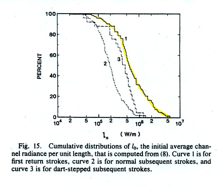
Actual measurements of mean radiance per unit length. A return stroke velocity of 8 x 107 m/s was assumed. Discharges were 5 to 35 km from the measuring site.