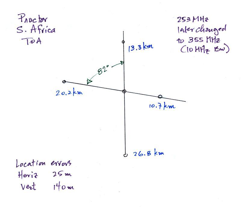
Probably the first 3-D TOA location system used for lightning research was D.E. Proctor's South African network. It is shown below and is described in more detail in Proctor (1971). This is a long baseline system where the distance between receivers (a few 10s of km in this case) is much greater than the wavelength of the VHF radiation.
In Proctor's sytem, four 253 MHz receivers (later changed to 355 MHz) were positioned at the ends of two nearly perpendicular baselines. A fifth receiver was positioned in the center at the intersection of the two baselines. Signals received at the four outer stations were transmitted to the center station by microwave link. Because the time of propagation from the outer stations to the center station could be accurately determined, the time of the arrival of signals at the outer stations could be determined very precisely.
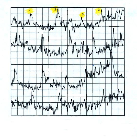
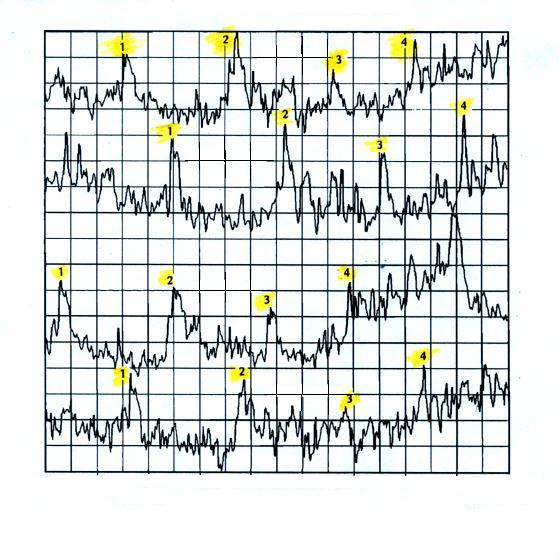
An example of RF data from the 5 receivers is shown below (from Proctor, 1983). The records are approximately 60 microseconds long.
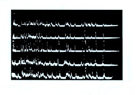
Initially the RF data from the 5 stations was recorded on a cathode ray tube and photographed (a "laser optical recorder" was later used to record the data on film). In the example above, the data recorded on film have been digitized and displayed on a computer.
In order to locate an emission source in space you must first identify the correlated RF impulses on the 5 records. The records can be complex with signals from multiple sources arriving at the different receivers in different order. This analysis was originally done by hand and could be quite tedious (the following quotes are from Proctor 1981)
"Even those who enjoy reading reading records that can be deciphered easily found that reading the more complicated variety was a mild from of torture, and that it took about one man-month's effort to locate 100 sources correctly."
On average it was possible to locate the source of one pulse in every 70 microseconds of record.
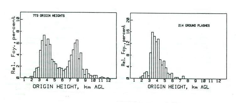
We'll look at an interesting example of results obtained with the South African VHF TOA network. Proctor (1991) determined where lightning discharges began by finding the centroid of the first 6 to 10 VHF pulse locations emitted in a flash. The left figure below shows origin heights (above ground level) for 773 cloud-to-ground and intracloud flashes in 13 thunderstorms. Origin heights for 214 cloud-to-ground flashes are shown in the figure at right. The network was 1.43 km above sea level.
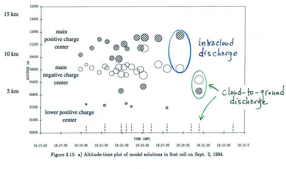
We can refer back to a figure in Lecture 12 (reproduced below) showing the locations of charge centers involved in cloud-to-ground and intracloud discharges (the charge center locations where derived from E field change measurements made at multiple sites using the field mill network at the Kennedy Space Center).
Next we'll briefly discuss another long baseline VHF TOA network, the Lightning Detection and Ranging (LDAR) system, that has been operating at the NASA Kennedy Space Center since the mid 1970s. The network has undergone several changes and upgrades since it was first installed. The figure below shows the layout of the system that was being used in the 1990s. It consisted of a central station and 6 surrounding stations positioned on roughly a 20 km diameter circle.
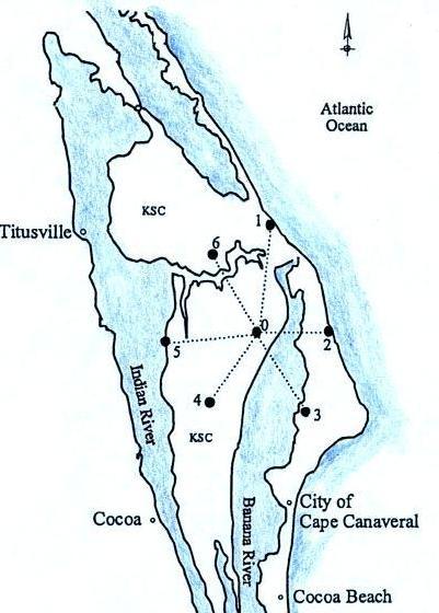
The VHF receivers operate at 66 MHz (6 MHz bandwidth) and data from the remote stations are telemetered back to the center station by microwave link where they are digitized. A signal crossing threshold at the center receiver triggers a roughly 100 μs; long recording at each of the 7 stations. Correlated pulses on the separate records and differences in the times of arrival are found using pattern recognition and cross correlation techniques TOA data from the center station and 3 of the outer stations (stations 0, 1,3, and 5 for example) are used to determine an RF source location. A second location is determined using the center data and the other 3 remote locations (stations 0, 2, 4 and 6). If the two locations agree the location is accepted.
Here is an example of VHF source locations provided by the LDAR network (from Rustan et al., 1980).
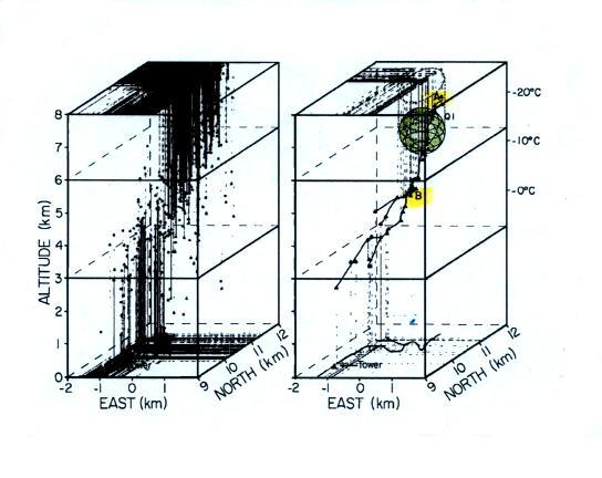
VHF noise began 4.9 ms before the 1st return stroke. The first 2.2 ms was considered preliminary breakdown actitivity and was followed by the stepped leader which lasted 2.7 ms. The left figure above shows 422 noise sources located during the first 4.7 ms of the flash. The right figure plots locations at 94 μs intervals during the preliminary breakdown (between Pts. A & B which are highlighted in yellow) and the stepped leader (below Pt. B). Q1 is the charge transported to ground during the first return stroke in this flash (determined from field change records using the methods discussed in Lecture 12). Four additional plots like this tracing out activity during the remainder of the discharge can be found in Rustan et. al (1980).
We'll next consider the most recent and most advanced VHF TOA system, the Lightning Mapping Array (LMA) developed by researchers at the New Mexico Institute of Mining and Technology (New Mexico Tech).
The system was originally used in Oklahoma in June 1998 (a map of sensor locations can be found here and results from the Oklahoma field experiment can be found here or here) and then in New Mexico in August and September. The New Mexico network, as described by Rison et. al (1999), consisted of 10 stations that were deployed over an area about 60 km in diameter near Langmuir Laboratory. Quoting from the Rison et. al article: "The time and magnitude of the peak radiation is recorded during every 100 μs time interval that the RF power exceeds a noise threshold." The time of the peak signal is recorded with 50 ns resolution. TOA information from events strong enough to be detected at six or more stations are located in space and time.
It is a little difficult to keep up with the rapid development and results coming from the LMA. As best I can tell (source) permanent and operational LMAs can be found at the NASA Marshall Space Flight Center in Alabama (see also this article), the National Weather Service in Washington DC, The National Severe Storms Lab in Norman OK, White Sands Missle Range in New Mexico, Dugway Proving Grounds in Utah, in Catalonia Spain, and Texas Tech University in Lubbock. Displays of real time data are available online at many of these sites.
Some photographs of an early version of the system being demonstrated in the Washington DC area are shown below (source of these images)
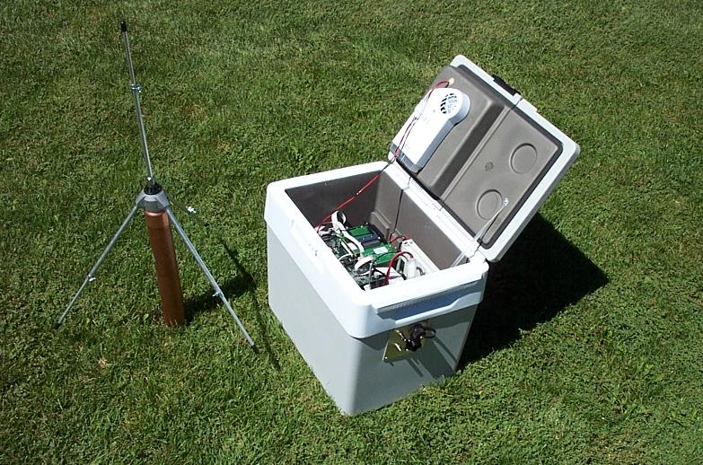
VHF antenna and open electronics enclosure showing the electronics (a more detailed photograph of the electronics can be found here)
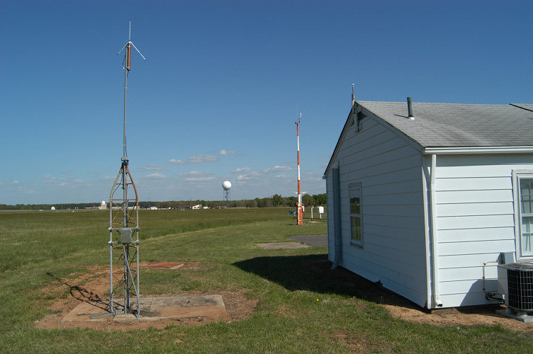
VHF antenna installation at the Sterling VA location.
Electronics enclosure.
Here are some animations of lightning activity located with the Oklahoma LMA. The links and explanation of the format of the data display below have been copied from http://lightning.nmt.edu/nmt_lms/ok98.html.
|
 The top t vs. z plot shows all the points located in the given time interval. The time is given in seconds, and the altitude z of the radiation source is given in kilometers. The number of points can be limited if desired. For example, two distinct discharges at different locations could occur at the same time, so the operator may choose to look at only one of the dishcarges in detail. Or the operator may narrow in on a particular event in time which he does not want obsured by other data points. The lower four plots show data points from the top plot which have been selected for such reasons. The lower t vs. z plot shows the time development of the altitude of the selected points. The x vs. y plot shows a plan view of the lightning discharge, where x is the distance east or west of the center of the array, and y is the distance north or south of the center. All distances are given in kilometers. The small squares in the x vs. y plot show the locations of the LMA stations. The x vs. z and y vs. z plots show the projections of the points on the xz and yz planes. Discharge showing distinct
charge layers at different
elevations.
Note the development of the dendritic structure of the discharge.
11 June 1998 06:33:20 UTC (645 KB Animated GIF) Cloud-to-ground discharge
followed by intercloud discharge.
Note the
well-defined leaders in the CG. The triangles are locations and times
of CG
strokes as determined by the National Lightning Detection Network. Note
that,
in the CG, positive streamers propagate in the negative charge region,
radially
away from the area of initial breakdown. The subsequent IC develops
over the
top of of the CG.
11 June 1998 06:19:39 UTC (1.5 MB Animated GIF)
Discharge near the end of a
storm which appears to be
inverted. There
are two distinct charge layers, but streamers appear to originate in
the upper
layer and propogate to the lower layer. This is inverted from most
intercloud
discharges in which negative streamers originate in the lower negative
charge
layer and propogate into the upper positive charge layer. Also note how
the
lower charge region decreases in altitude to the east.
20 June 1998 03:43:45 UTC (1.8 MB Animated GIF) |
Finally, be sure to look at this very cool animation of a lightning flash over New Mexico near Langmuir Lab that is on YouTube.
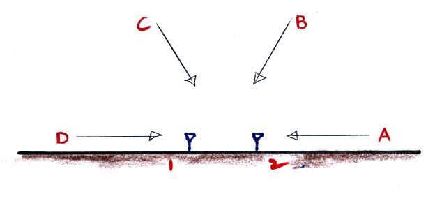
Interferometry is a different way of locating a source of VHF radiation emitted by lightning. The basic principle is shown below.
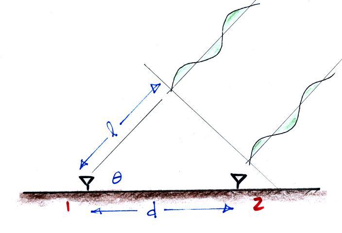
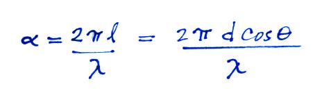
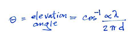
A plane wave of radiation is approaching from the right in the same direction as a line connecting two antennas on the ground. The antennas are a distance d apart. Radiation will arrive at Antenna 2 first. The radiation arriving at Antenna 1 travels an additional distance, l, before reaching the antenna. The interferometer measures the phase difference, α, in the signals arriving at the two antennas.
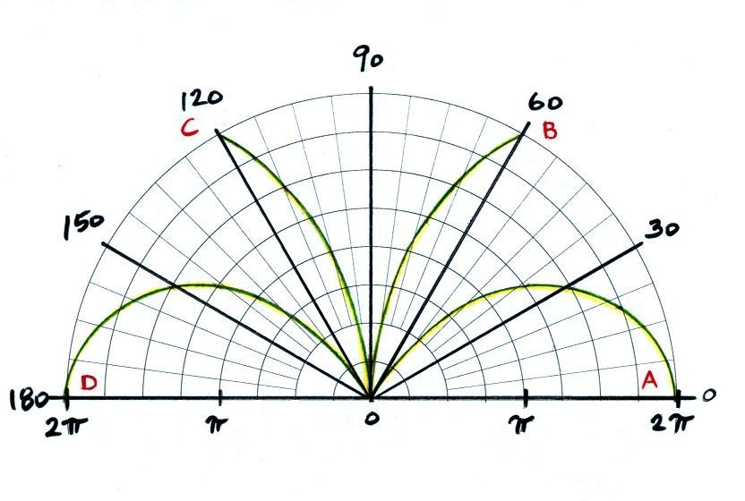
To illustrate the problem of multiple elevation angles for a given value of phase angle we draw the figure polar plot for a larger antenna separation, d = 2 λ.
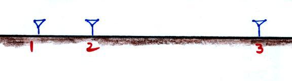
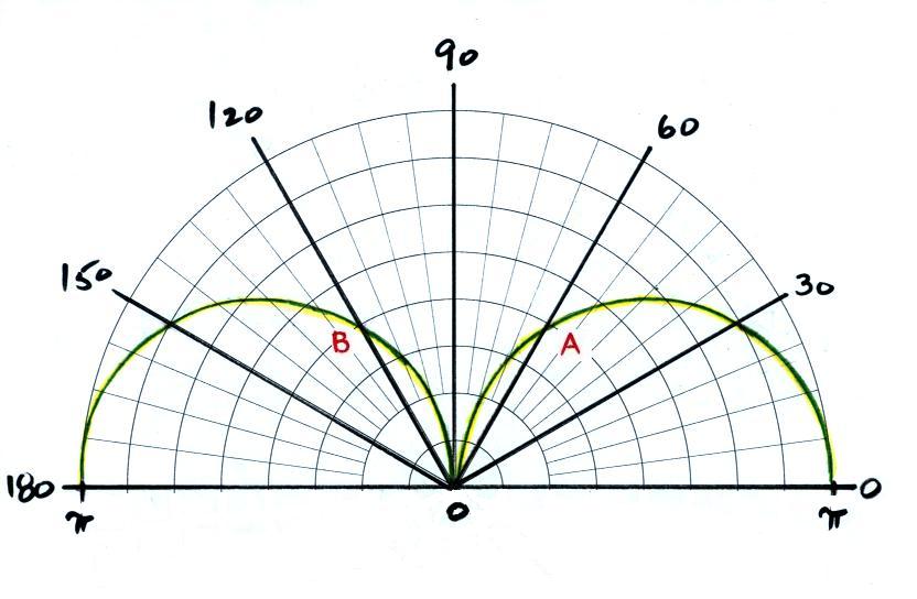
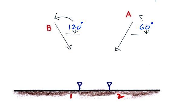
Up to this point we've been assuming that the direction of the incoming radiation is parallel to the baseline connecting the antennas (i.e. zero azimuth angle). There is no reason for that to be the case. As the azimuth angle moves from zero, the measured phase difference will begin to decrease. The phase angle difference will become zero for a signal approaching from a direction that is perpendicular to the baseline connecting the antennas. So to be able to determine the true direction angle to the emission source we're going to need a 2nd perpendicular baseline. Antenna 1 above can be part of both baselines. So we'll end up with something like shown below.
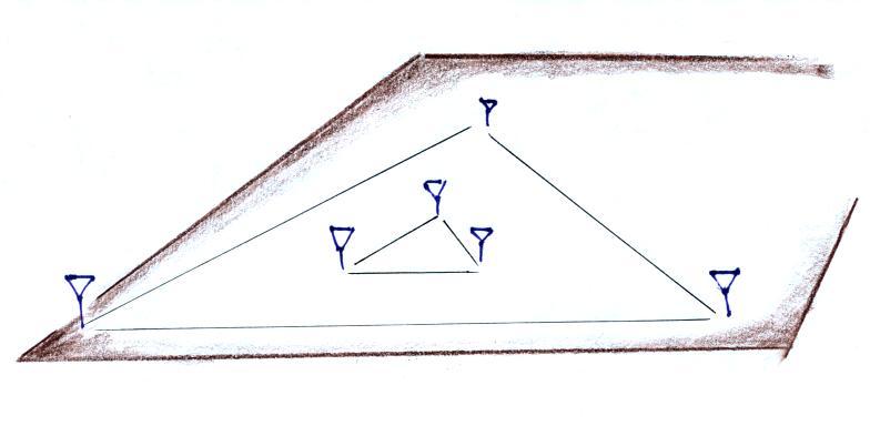
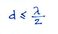
Richard et. al (1986) used 6 antennas arranged in a triangular pattern as shown above. Spacing between the inner antennas was either λ/2 or λ. Spacing between antennas in the outer triangle was 10λ (more than 250 ambiguous elevation angle values).
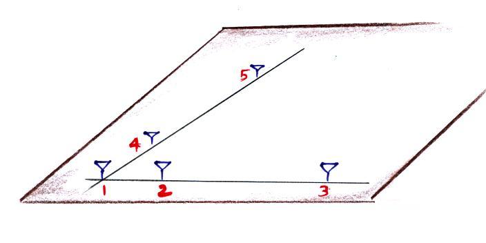
Now, as the next figure below suggests (adapted from Hayenga and Warwick, 1981), with two baselines you have sufficient data to determine the direction (azimuth and elevation angles) to the source of RF radiation.
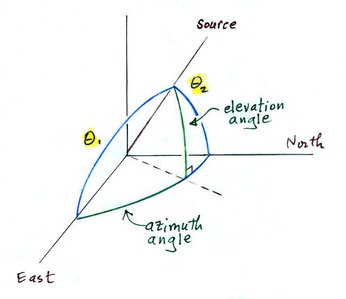
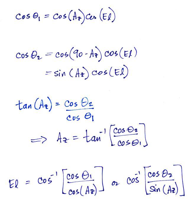
Note that a group of 5 or 6 antennas as sketched above just gives you the direction to the radiation source (elevation and azimuth angles but not the distance to the source). To actually locate the source in space, a second group (at least) of 5 antennas on perpendicular baselines at a different location would be needed.
And finally a brief comparison of lightning source locations from a TOA system (the LDAR network operating at the Kennedy Space Center) and an interferometer developed by the French Office National D'Etudes et de Recherches Aerospatiales (ONERA). The ONERA system was operated near Orlando, about 60 miles from the Kennedy Space Center in 1992 and 1993. The results we will be discussing are from Mazur et. al (1997).
We mentioned at the beginning of the previous lecture that TOA systems are best able to locate sequences of narrow (pulse widths on the order of microseconds), isolated pulses that are emitted at relatively low repetition rates (1 to 100 pulses per millisecond). Interferometers are better able to locate the sources of more quasi continuous emissions such as are produced by dart leaders and recoil streamers.
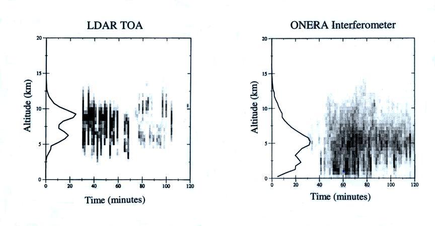
Even though we're not looking at observations of the same storm we can draw some conclusions. The greatest source density for the LDAR data falls between about 6 km and 10 or 11 km which is higher than the ONERA locations where peak density is between the ground and about 7 km. Radiation sources mapped by the LDAR system remain in the cloud and do not extend to the ground as happens with the ONERA data.
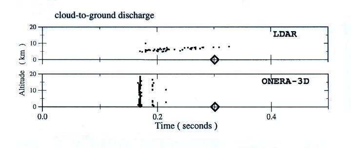
Simultaneous observations of individual discharges by both locating systems were available for only one storm (the Aug. 28, 1993 storm). An example of an intracloud and a cloud-to-ground discharge are shown below.
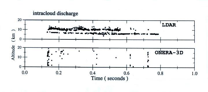
Radiation sources are mapped almost continuously during the discharge by the LDAR system. Source locations also appear in two distinct layers. This is similar to what Proctor (1991) found when locating the first emissions sources that occur in a discharge.
The sources mapped by the ONERA system appear intermittently with quiet periods in between. You might be bothered by the fact that the ONERA system shows locations extending down to ground level during an intracloud discharge. This storm was well outside the nominal range of the ONERA system so the location accuracy is poor. Both the high source locations (near 20 km) and locations near the ground are due to location errors. The intracloud discharge did not produce channels that extended down to the ground.
Clearly there are differences in the picture of lightning flashes presented by TOA systems and interferometers. Mazur et. al (1997) suggests this is "because most of the radiation sources mapped with LDAR are associated with virgin breakdown processes typical of slowly moving negative leaders. On the other hand, most of the radiation sources maped with ONERA-dD are produced by fast intermittent negative breakdown processes typical of dart leader and K charnges as they traverse the previously ionized channgels. Thus each operational system may emphasize different stages of the lightning flash, but neither appears to map the entire flash."
Mazur, V., E. Williams, R. Boldi, L. Maier, D.E. Proctor, "Initial comparison of lightning mapping with operational Time-Of-Arrival and Interferometric systems," J. Geophys. Res., 102, 11071-11085, 1997.
Proctor, D.E., "A Hyperbolic System for Obtaining VHF Radio Pictures of Lightning," J. Geophys. Res., 76, 1478-1489, 1971.
Proctor, D.E., "VHF Radio Pictures of Cloud Flashes," J. Geophys. Res., 86, 4041-4071, 1981.
Proctor, D.E., "Lightning and Precipitation in a Small Multicellular Thunderstorm," J. Geophys. Res., 5421-5440, 1983.
Proctor, D.E., "Regions Where Lightning Flashes Begin," J. Geophys. Res., 96, 5099-5112, 1991.
Rhodes, C.T., X.M. Shao, P.R. Krehbiel, R.J. Thomas, and C.O. Hayenga, "Observations of lightning phenomena using radio interferometry," J. Geophys. Res., 13059-13082, 1994.
Richard, P., A. Delannoy, G. Labaune, and P. Laroche, "Results of Spatial and Temporal Characteristics of the VHF-UHF Radiation of Lightning," J. Geophys. Res., 91, 1248-1260, 1986.
Rison, W. R.J. Thomas, P.R. Krehbiel, T. Hamlin, and J. Harlin, "A GPS-based Three Dimensional Lightning Mapping System: Initial Observations in Central New Mexico," Geophys. Res. Lett., 26, 3573-3576, 1999.
Rustan, P.L., M.A. Uman, D.G. Childers, and W.H. Beasley, "Lightning Source Locations From VHF Radiation Data for a Flash at Kennedy Space Center," J. Geophys. Res., 85, 4893-4903, 1980.
Uman, M.A., W.H. Beasley, J.A. Tiller, Y-T. Lin, E.P. Krider, C.D. Weidman, P.R. Krehbiel, M. Brook, A.A. Few, J.L. Bohannon, C.L. Lennon, H.A. Poehler, W. Jafferis, J.R. Gulick, J.R. Nicholson, "An Unusual Lightning Flash at Kennedy Space Center," Science, 201, 9-16, 1978.