It is essential that we have an
accurate idea of average and extreme
lightning current parameters such as Ipk
and (dI/dt)pk in order to design
effective lightning protection. In
this
lecture we will learn how
certain lightning return
stroke current characteristics might be estimated from remote
measurements of E and B fields. It is much easier to make
remote
measurements of lightning electric and magnetic fields than it is to
make
direct measurements of lightning return stroke currents.
This will first involve learning something
about the
fields radiated by lightning and about how return stroke currents might
vary with
time and altitude along the lightning channel.
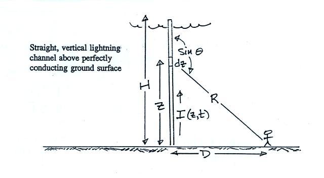
First here's the geometry used in
the E and B fields calculations that follow. We aren't going to
look at all the steps in the
derivation, we'll simply write down the results.
If you are interested in the details a good place to start would be the
following article: "The
Electromagnetic
Radiation
from
a
Finite
Antenna,"
M.A.
Uman,
D.K.
McLain,
and
E.P.
Krider,
Am.
J.
Phys.,
43
33-38,
1975.
The lightning channel is assumed to be straight and vertically oriented. The expression below gives the electric field radiated by a short segment dz located at an altitude z above the ground. We'll limit our attention to the E field at the ground (assumed to be a perfect conductor) which has just a z component. There is interest in how lightning E and B fields couple onto electric power lines. To properly examine this problem you would need to compute E and B for points above the ground (at the level of the power lines). That becomes a more complicated problem because the E and B fields will each have 3 components (vertical, radial, and azimuthal components in cylindrical geometry).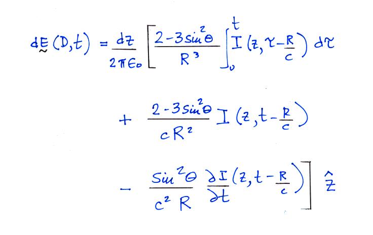
The lightning channel is assumed to be straight and vertically oriented. The expression below gives the electric field radiated by a short segment dz located at an altitude z above the ground. We'll limit our attention to the E field at the ground (assumed to be a perfect conductor) which has just a z component. There is interest in how lightning E and B fields couple onto electric power lines. To properly examine this problem you would need to compute E and B for points above the ground (at the level of the power lines). That becomes a more complicated problem because the E and B fields will each have 3 components (vertical, radial, and azimuthal components in cylindrical geometry).
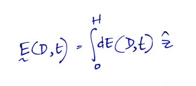
To obtain the total E field we need
to integrate from the ground to the top of the channel
At the ground the magnetic field has just an azimuthal component
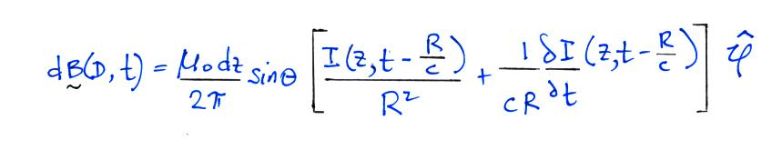
and again we integrate over the length of the channel to determine
the total field.

I should mention also that there is
a small error in the
expressions
above. This won't affect our discussion, but if you would like to
see the correct expressions, click here.
We won't really be using these rather complex general expressions very much. Rather let's just note that the electric field expression contains terms involving a time integral of current, the current itself, and a time derivative term.
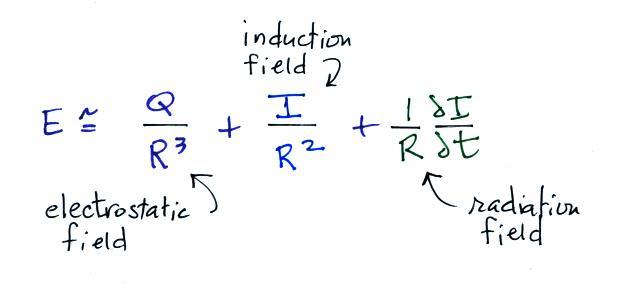
We refer to these are the electrostatic, induction, and
radiation field components. The B field has just induction and
radiation field components.
The electrostatic field is generally dominant at close range. Because it decreases as 1/R, the radiation field is the only field component observed at long range (beyond a few 10s of kilometers). Also because peak dI/dt occurs very early in a return stroke discharge, the radiation field also dominates at the very beginning of a return stroke.
The figure below provides a rough idea of the what the 3 field components would look like given the current waveform at the top of the figure.
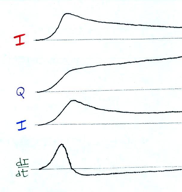
The solid lines show typical first return field values, the dotted
lines are for subsequent strokes. These aren't actual
waveforms. Rather they are essentially an average of measurements
of actual waveforms
(lots of
waveforms).
The hump on these magnetic fields is probably coming from the induction field. We don't see it on E field waveforms because the electrostatic field component dominates. B fields don't have a magnetostatic field component.
The E and B fields at a particular distance from a lightning strike depend in a complex way on return stroke current, the current derivative, and, for E fields, on the time integral of the current. We really don't know what the return stroke current is as a function of altitude and time [ that is, I(z,t) ]. At best we can sometimes measure I(0,t) [i.e. the current at the ground in triggered lightning discharges, for example].
Let's remember that what we are hoping to do is to measure E and/or B and go back and figure out what the return current must have been. In order to do that we will need to make some assumptions or put some constraints on the return stroke current. We will need a lightning return stroke "current model."
We can roughly classify current models into 3 groups:
1. Sophisticated plasma-fluid-dynamics models that try to realistically determine the actual physical conditions in a lightning channel (temperature, electron density, pressure, and other electrical and fluid properties). This type of approach is beyond the scope of this class.
2. Because the lightning return stroke current begins at (or near) the ground and travels upward along a conducting channel, many researcher treat the return stroke as a voltage or current pulse traveling along a transmission line with distributed resistance, inductance, and capacitance.
We will adopt the following approach
3. We will assume a functional form for I(z,t), calculate the E and B field that such a current would produce, and then compare the calculations with field measurements (often made at two distances from the return stroke). We will then adjust I(z,t) to get the best agreement between calculated and measured fields.
Bruce Golde Model
In the Bruce Golde model the return stroke current is assumed to
be uniform along the length of the channel. The current
amplitude can change with time but it does so along the entire length
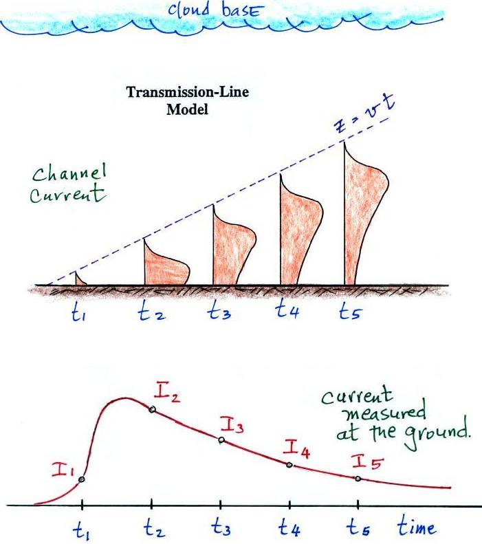
of the channel simultaneously. This is illustrated further in the
figure below which shows the height of the return stroke
channel and the
current distribution along the channel at evenly spaced time intervals t1
through t5.

The current waveform measured at the ground is shown at the bottom of the figure. The top part of the figure shows the upward development of the channel. The height and current distribution is shown at evenly spaced time intervals. The width of each vertical bar indicates the current amplitude. As the current amplitutde is changing at the ground with time, current amplitude also changes simultaneously along the entire length of the channel. This is physically unreasonable as it would require that information propagate along the length of the channel at infinite speed.
We won't really be using these rather complex general expressions very much. Rather let's just note that the electric field expression contains terms involving a time integral of current, the current itself, and a time derivative term.
The electrostatic field is generally dominant at close range. Because it decreases as 1/R, the radiation field is the only field component observed at long range (beyond a few 10s of kilometers). Also because peak dI/dt occurs very early in a return stroke discharge, the radiation field also dominates at the very beginning of a return stroke.
The figure below provides a rough idea of the what the 3 field components would look like given the current waveform at the top of the figure.
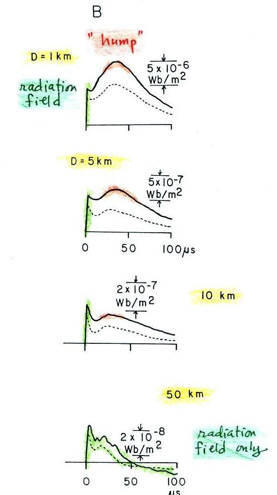
And here are more realistic shapes
of E and B
waveforms that you might expect to see at various
distances from a CG stroke (source: Lin,
Y.T.,
M.A.
Uman,
J.A.
Tiller,
R.D.
Brantley, W.H. Beasley, E.P. Krider,
C.D. Weidman, "Characterization of Lightning Return Stroke Electric and
Magnetic Fields from Simultaneous Two-Station Measurements," J.
Geophys. Res., 84-6307-6314, 1979).
.

.
The hump on these magnetic fields is probably coming from the induction field. We don't see it on E field waveforms because the electrostatic field component dominates. B fields don't have a magnetostatic field component.
The E and B fields at a particular distance from a lightning strike depend in a complex way on return stroke current, the current derivative, and, for E fields, on the time integral of the current. We really don't know what the return stroke current is as a function of altitude and time [ that is, I(z,t) ]. At best we can sometimes measure I(0,t) [i.e. the current at the ground in triggered lightning discharges, for example].
Let's remember that what we are hoping to do is to measure E and/or B and go back and figure out what the return current must have been. In order to do that we will need to make some assumptions or put some constraints on the return stroke current. We will need a lightning return stroke "current model."
We can roughly classify current models into 3 groups:
1. Sophisticated plasma-fluid-dynamics models that try to realistically determine the actual physical conditions in a lightning channel (temperature, electron density, pressure, and other electrical and fluid properties). This type of approach is beyond the scope of this class.
2. Because the lightning return stroke current begins at (or near) the ground and travels upward along a conducting channel, many researcher treat the return stroke as a voltage or current pulse traveling along a transmission line with distributed resistance, inductance, and capacitance.
We will adopt the following approach
3. We will assume a functional form for I(z,t), calculate the E and B field that such a current would produce, and then compare the calculations with field measurements (often made at two distances from the return stroke). We will then adjust I(z,t) to get the best agreement between calculated and measured fields.
We'll mostly just discuss two well
know current models: the Bruce-Golde and the Transmission Line models.
Bruce Golde Model
The current waveform measured at the ground is shown at the bottom of the figure. The top part of the figure shows the upward development of the channel. The height and current distribution is shown at evenly spaced time intervals. The width of each vertical bar indicates the current amplitude. As the current amplitutde is changing at the ground with time, current amplitude also changes simultaneously along the entire length of the channel. This is physically unreasonable as it would require that information propagate along the length of the channel at infinite speed.
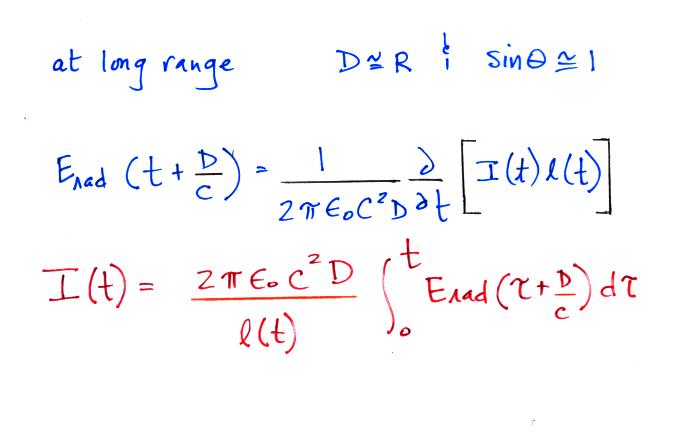
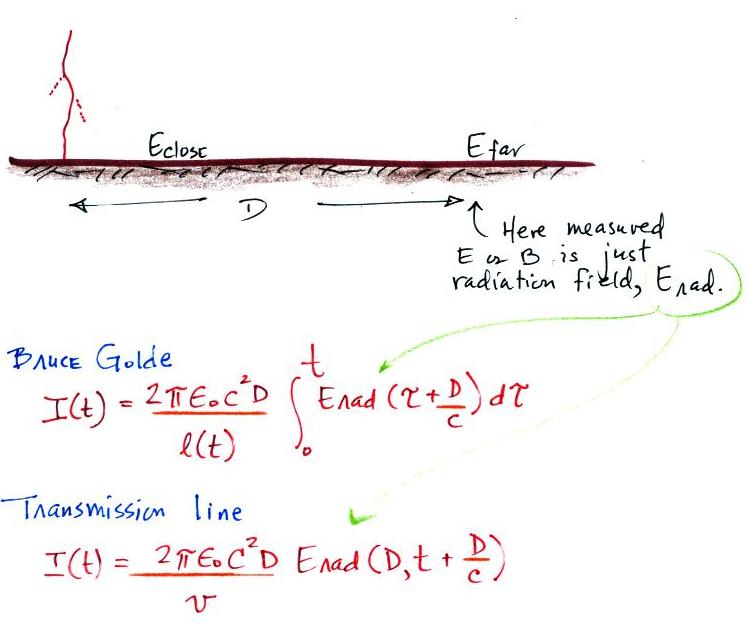
Here is first an expression for the
radiation field component of
the electric field (Erad) at a
distance D from the lightning
stroke.
There are a few tricks involved in this derivation (that we won't worry
about) because the current is discontinuous at the tip of the
upward propagating return stroke current. The expression for E
can be inverted to give the channel base current as a function of
the field (the last equation in the figure above).
Transmission Line Model
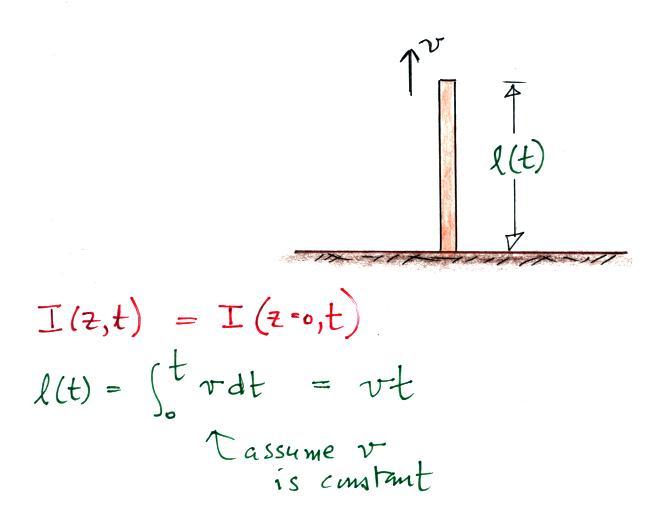
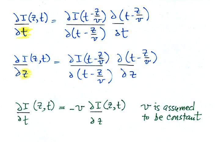
In the transmission line model the current waveform measured at the ground is assumed to propagate up the channel without changing shape and at constant speed. Here's how that is expressed in equation form.
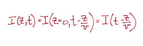
Basically the current value observed at height z at time t is the same as the current seen at the ground at a time (t - z/v) earlier (i.e. the time it took to travel from the ground up to height z). Again this might be clearer in picture form.
The current waveform measured at the ground propagates up the channel without changing shape or speed.
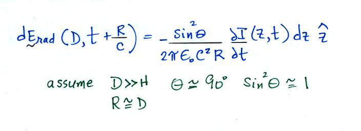
The radiation field produced by a segment dz of channel located at height z above the ground is shown below
Transmission Line Model
In the transmission line model the current waveform measured at the ground is assumed to propagate up the channel without changing shape and at constant speed. Here's how that is expressed in equation form.
Basically the current value observed at height z at time t is the same as the current seen at the ground at a time (t - z/v) earlier (i.e. the time it took to travel from the ground up to height z). Again this might be clearer in picture form.
The current waveform measured at the ground propagates up the channel without changing shape or speed.
The radiation field produced by a segment dz of channel located at height z above the ground is shown below
Because of the functional form of
I(z,t), we can replace the partial derivative with respect
to time with a partial with respect to z.
This
makes it easy to integrate over z.
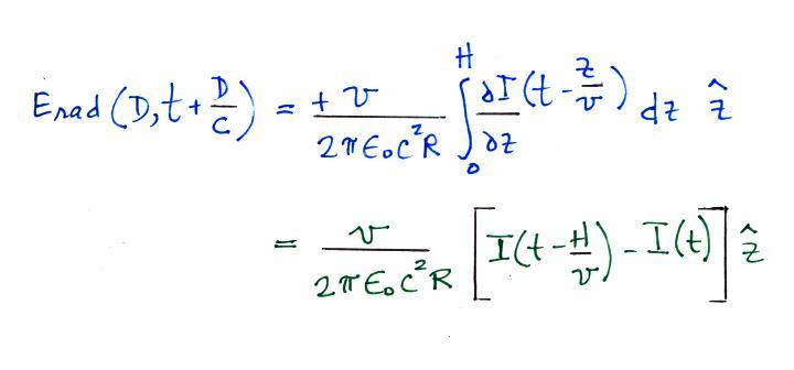
H is the height of the return stroke channel. The first term in brackets is zero at times less than H/v (i.e. before the return stroke tip reaches the top of the channel).
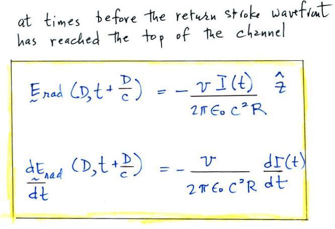
H is the height of the return stroke channel. The first term in brackets is zero at times less than H/v (i.e. before the return stroke tip reaches the top of the channel).
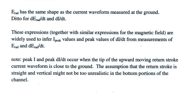
You couldn't ask for a simpler
relationship between E and I (or dE/dt and dI/dt).
Now we'll look at an experimental
test of the Bruce Golde (BG) and Transmission Line (XL)
models.
Measurements of electric and
magnetic fields were
measured at 2 stations: one close to and the other far from the strike
point. The far field measurements (which are just radiation
fields
and don't contain any induction or electrostatic fields) were used to
determine the return stroke channel current, I(t), using of the two
equations above. Then both near and far fields were calculated
and compared with the
actual measurements at the two sites.
Here are some of the results from the tests. In this case the distant station (the Kennedy Space Center, Florida) was 200 km from the lightning strike point, the close station (Gainesville, Florida) was only 2 km away. These data are from "Lightning Return Stroke Models," Y.T. Lin, M.A. Uman, and R.B. Standler, J. Geophys. Res., 85, 1571-1583, 1980.
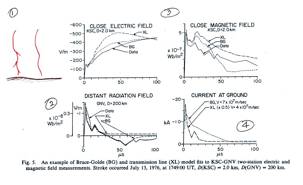
Point 1. The experimental tests used only the fields from subsequent strokes because, without branches, they are closer to the model assumptions that the lightning channel is straight and vertical. A constant return stroke propagation speed was assumed and the value was adjusted to give the best fit between measured and computed fields.
Point 2. Note first the measured distant E radiation field is labeled "Data" on the graph. This field is used in the Bruce Golde (BG) and Transmission line (XL) models to derive the return stroke current I(z,t) (the derived currents are shown at Point 4). Then the E radiation fields are computed using both the BG and TL currents. You can see for the distant fields, the agreement is pretty good but not perfect. In particular the XL calculated field never goes below zero.
Point 3. The derived currents were then used to compute the E and B fields at the closer station. The calculated fields were then compared to the measured fields. The agreement wasn't particularly good.
Point 4. The derived currents are plotted. The XL model current waveform is too narrow and is unrealistic.
Here are some of the results from the tests. In this case the distant station (the Kennedy Space Center, Florida) was 200 km from the lightning strike point, the close station (Gainesville, Florida) was only 2 km away. These data are from "Lightning Return Stroke Models," Y.T. Lin, M.A. Uman, and R.B. Standler, J. Geophys. Res., 85, 1571-1583, 1980.
Point 1. The experimental tests used only the fields from subsequent strokes because, without branches, they are closer to the model assumptions that the lightning channel is straight and vertical. A constant return stroke propagation speed was assumed and the value was adjusted to give the best fit between measured and computed fields.
Point 2. Note first the measured distant E radiation field is labeled "Data" on the graph. This field is used in the Bruce Golde (BG) and Transmission line (XL) models to derive the return stroke current I(z,t) (the derived currents are shown at Point 4). Then the E radiation fields are computed using both the BG and TL currents. You can see for the distant fields, the agreement is pretty good but not perfect. In particular the XL calculated field never goes below zero.
Point 3. The derived currents were then used to compute the E and B fields at the closer station. The calculated fields were then compared to the measured fields. The agreement wasn't particularly good.
Point 4. The derived currents are plotted. The XL model current waveform is too narrow and is unrealistic.
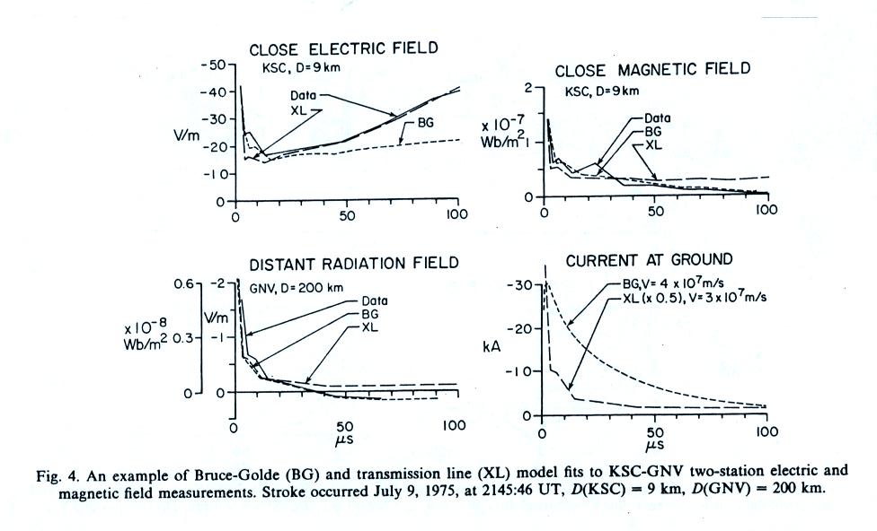
An additional set of test results
(the lightning strike was 9 km from the measuring site at the Kennedy
Space Center and 200 km from the measuring station at the University of
Florida in Gainesville).
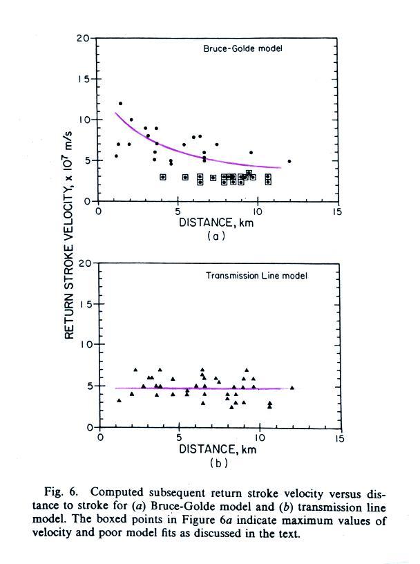
A return stroke velocity was determined for each set of near and far E and B field measurements (the velocity value was the one that provided the best fit between measured and calculated fields). The velocity values derived for the BG model are shown in the top graph and appear to be distance dependent (distance from the close station to the lightning strike point). That is a physically unreasonable result. The velocities derived for the TL model appear in the bottom plot. The values are more reasonable; perhaps a little lower than the 1 x 10⁸ m/s commonly assumed for return strokes but at least they do not appear to vary with distance.
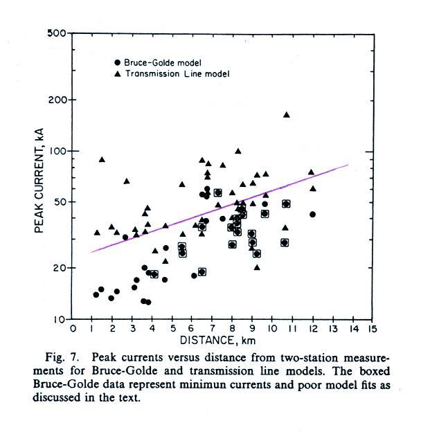
Here are the peak current values derived for both the TL and BG
models. In both cases peak current values appear to be distance
dependent which is not realistic. Many of the TL peak currents
are too large. First return stroke peak currents are typically
about 30 kA. Subsequent stroke peak currents are usually
less. Some of the TL peak currents in the plot above exceed 100
kA.
A return stroke velocity was determined for each set of near and far E and B field measurements (the velocity value was the one that provided the best fit between measured and calculated fields). The velocity values derived for the BG model are shown in the top graph and appear to be distance dependent (distance from the close station to the lightning strike point). That is a physically unreasonable result. The velocities derived for the TL model appear in the bottom plot. The values are more reasonable; perhaps a little lower than the 1 x 10⁸ m/s commonly assumed for return strokes but at least they do not appear to vary with distance.
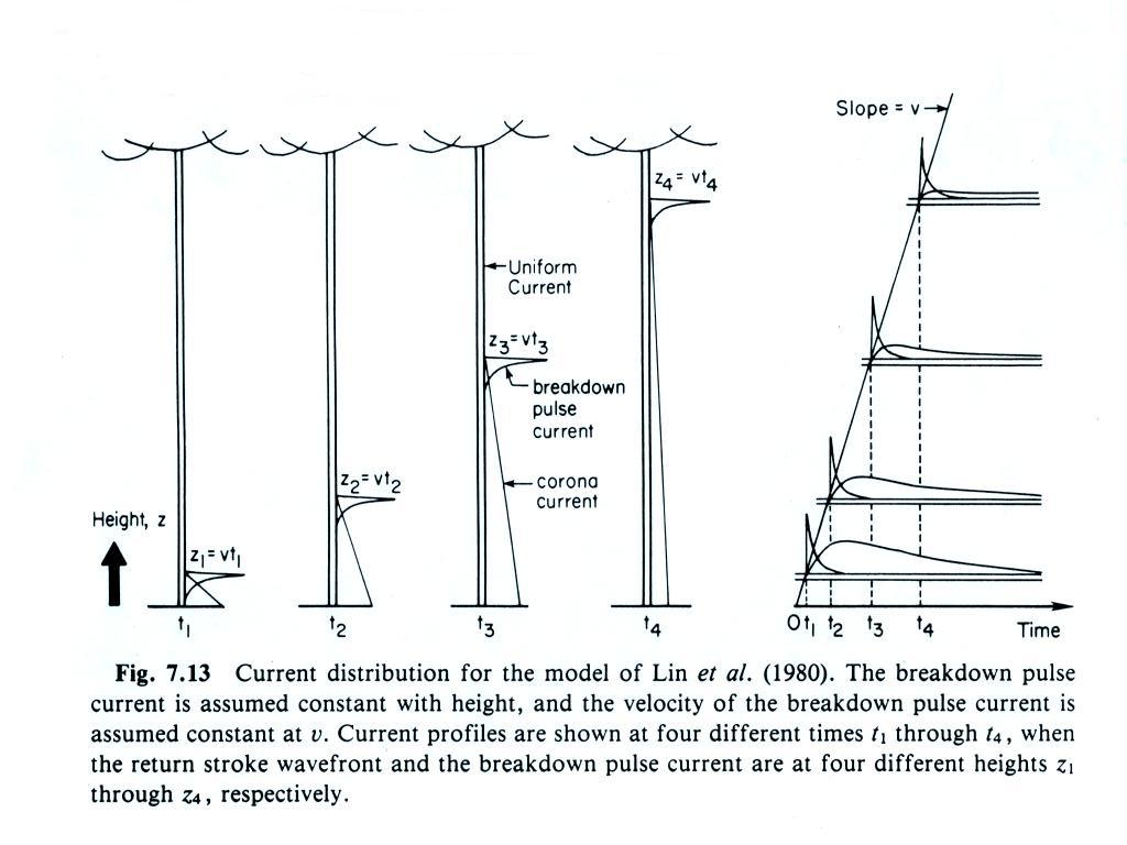
Neither the transmission line or
the Bruce-Golde did a very good job of reproducing the measured fields,
particularly at close range. The researchers that conducted these
experimentals tests made some changes to the assumed return stroke
current. In particular they found that 3 current components were
needed to better reproduce the near fields: a breakdown current, a
corona current and a uniform current. (source: Uman, M.A., The
Lightning Discharge, Academic Press, Orlando, 1987, see also the Lin,
Uman, and Standler (1980) reference mentioned earlier).
We won't discuss this further in this class as we'll mostly be interested in estimating peak I and peak dI/dt values from measurements of radiation fields. And in that case it looks like the transmission line model does a pretty good job. We'll look at this further in Lecture 18.
We won't discuss this further in this class as we'll mostly be interested in estimating peak I and peak dI/dt values from measurements of radiation fields. And in that case it looks like the transmission line model does a pretty good job. We'll look at this further in Lecture 18.