Lecture 16

The topic of this lecture is lightning return stroke currents.  We'll look at what current properties or parameters are of interest (mostly from a lightning damage or protection point of view) and look at measurement techniques.  In Lecture 17 we'll look at how return stroke currents can be determined from remote measurements of the electromagnetic fields radiated by lightning.

We'll cover most of the material listed on the outline below (normally distributed on a handout in the lecture version of this course).


We'll start with some examples of situations where lightning current parameters such as peak current amplitude or peak current derivative value are of interest.  Then we'll will look at some of the techniques, both older and more modern, that are used to measure lightning current directly.  The reference listed noted on the figure can be found at the end of today's notes.


Now a quick look at the engineering parameters and examples of situations where they are important. 

Peak current is of interest when lightning strikes an object that presents a resistive load to the lightning current.  M.A. Uman, in his 2008 book "The Art and Science of Lightning Protection," uses the example of a phase conductor on a power line.  Power lines, apparently, have a characteristic impedance of about 500 ohms.


A 1st return stroke typically has a peak current of about 30,000 Amps.  Assume that the current divides in half as shown above and then travels through 500 ohms to ground.  This will produce a voltage of 15,000 Amps x 500 ohms = 7.5 Mvolts.  This is high enough to spark across to a ground wire or one of the other phase conductors (and once an arc is initiated it is sometime difficult to "turn off".

Lightning rods on the house sketched below are connected to ground rods that are driven into the soil. 


Depending on the soil type and moisture content, the ground resistance can range from a few 10s of ohms to a few 100s of ohms.  A peak current of 30,000 Amps would produce a voltage of 750,000 volts across 25 ohms and 7.5 Mvolts across 250 ohm.  The latter value almost certainly would be enough to spark across to nearby plumbing or something like that (the lightning rod should be electrically connected (bonded) to a nearby water pipe to avoid this kind of occurrence).


The peak value of the return stroke current derivative is of interest if lightning strikes something with an inductive impedance. 

The straight down conductor in the sketch above has an impedance, L, of roughly 1 microHenry per meter.  Lightning return strokes (both 1st and subsequent strokes) have peak current derivatives values of about 100 kA/μsec or about 1011 A/sec.
The voltage produced here will be L x dI/dt = 1011 A/sec x 10-6 H = 100,000 volts. 

The lightning dI/dt will produce a time varying magnetic field that can couple into nearby electronics (loops are of primary concern).


The time integral of the return stroke current gives the total charge transferred during the strike.  This apparently determines whether the lightning current will burn through a sheet of metal (such as a metal roof or the thin metal skin of an airplane).


The lightning will burn through the metal sheet unless heat can be carried away from the strike point quickly enough.   Not as much charge would be needed to burn through thin sheets because they won't be able to dissipate heat as quickly as thicker sheets.  Here it is the continuing currents that are of concern because that is where most of the charge transfer occurs.  I like to think of the lightning strike resembling an arc welder in cases like this. 

The last parameter of interest is called the action integral


The instantaneous power dissipated by a resistive load is


so the energy deposited is R times the action integral

This will cause heating or can cause vaporization of materials with low electrical conductivity that are struck.  Lightning can vaporize the sap in a tree, for example, and cause the tree to explode.


Some of the earliest estimates of return stroke peak currents come from measurements of the residual magnetism in nephelitic basalt (whatever that is) near trees that were struck by lightning (within centimeters of the tree perhaps).  The data were published by Pockels in 1897 & 1898 (the publications would be interesting to look at, unfortunately they are in German).

Pockels had determined, in laboratory experiments, that magnetization of the basalt depended on the peak current value along and wasn't affected by the shape of the current waveform or its duration. 

The sketch below shows a klydonograph.  A high voltage will produce a Lichtenberg figure on the film. 


The diameter of the pattern depends on the peak voltage which can then be related to peak current if the impedance of the arrangement is known. 


Different patterns are produced depending on the polarity of the applied voltage.
  Here's an informative web site with some interesting historical background on Lichtenberg figures.

A Lichtenberg figure like pattern is often burned into the grass after lightning strikes a golf course green.  Similar burn patterns are, apparently, sometimes seen on lightning strike victims.

"Magnetic links" have been used extensively by the electric power industry to estimate peak currents in lightning strikes to power lines.

A magnetizable material is positioned perpendicularly to a straight conductor.  The strength of the magnetization in the link can be related to the peak current in the conductor.  Often two or more links are mounted with different orientations and at different distances from the conductor.

An inexpensive version was at one time used at the Kennedy Space Center to estimate peak currents in certain launch facilities.  A strike to a launch complex would probably require time consuming and expensive testing to ensure the facility hadn't been damaged and was still fully operational. 


A loop of prerecorded magnetic tape (on a plastic support and sealed inside a length of  PVC pipe) was positioned perpendicularly to conductors that might carry large amplitude lightning currents.  A portion of the signal on the tape would be erased by the magnetic fields produced by lightning currents.  The magnetic tape wouldn't be removed and analyzed unless the photo bulb had flashed, indicating that a lightning strike had occurred.

A wire loop placed close to a straight conductor can be used to determine the current derivative.


This is the principle behind a Rogowski Coil used to measure time varying currents moving through a conductor.  Multiple loops of wire on a toroidal support surround the conductor.


The multiple loops of wire increases the inductance which limits the high frequency response of a sensor like this.

A sketch of a faster dI/dt sensor is shown below.

The induced voltage is measured across the gap on the inside surface of the sensor.  Sensors like this are used to measure lightning dI/dt signals and also are used in nuclear electromagnetic pulse testing.

Breaking the current conductor and adding an in-line resistive element is perhaps a more obvious way of measuring lightning currents.

Ideally then you would measure a voltage across the "shunt" that is simply R times I (R is the resistance of the shunt and I is the lightning current).  Very low resitance values (on the order of a milliohm) are needed because peak lightning current amplitudes are large. 

As the picture above shows however, measuring the voltage across the shunt introduces a loop circuit.  The lightning will produce a time varying magnetic field that will couple into the loop.  This will add an L dI/dt term to the output voltage.  Even if L is small, the lightning peak dI/dt can be very large.


The problem with induced voltages in the measuring circuit can be avoided if a coaxial shunt design is used.


Here's a crossectional view.  The resistive element has a cylindrical shape and the measuring circuit is inside the cylinder where the magnetic field is zero (B fields from currents flowing in the right and left hand sides of the cylinder point in opposite directions and cancel).  The measuring instrumentation is placed in the metal enclosure (rectangular or cylindrical), a Faraday cage, at the top part of the figure.  Signals could then be sent out on fiber optics cables to a nearby trailer for recording.
Current is shown flowing through one side of the diagram.  In reality it flows through all sides.

There can still be some problems with a coaxial shunt.  Large currents can heat the resistive element and change the resistance (or heat it so much that it is damaged).  Also high frequency currents may only flow through the skin and not through the entire volume of the resistive element and the actual resistance wouldn't be known.

A schematic illustration from one of the triggered lightning experiments in Florida (at the northern edge of the Kennedy Space Center in this case, not at the Univ. of Florida site.  Source: Leteinturier, C., J.H. Hamelin, A. Eybert-Berard, "Submicrosecond Characteristics of Lightning Return-Stroke Currents," IEEE Trans. EMC, 33, 351-357, 1991).

A coaxial shunt (I sensor in the figure) was positioned just below the Faraday cage (which containined the measuring equipment and also the electronics that controlled firing of the rockets).  A dI/dt sensor surrounds the lightning current conductor a little bit further down.  This launch platform was actually floating on brackish water.

The next figure  shows some examples of lightning I and dI/dt records from two strokes in a flash triggered during the 1988 experiments in Florida.


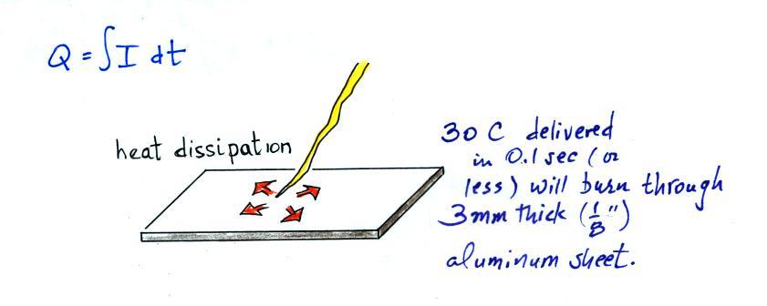
We'll finish this lecture with a quick look at some of the results from some of the triggered lightning 
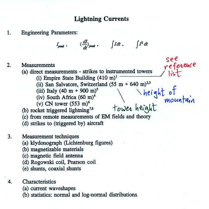
experiments and compare those results with data from some of the older lightning current measurements during lightning strikes to instrumented towers made in Switzerland and Italy. 

We'll spend most of the class period examining some of the work that has been done to try to determine lightning peak I and peak dI/dt values from remote measurements of E and B fields.


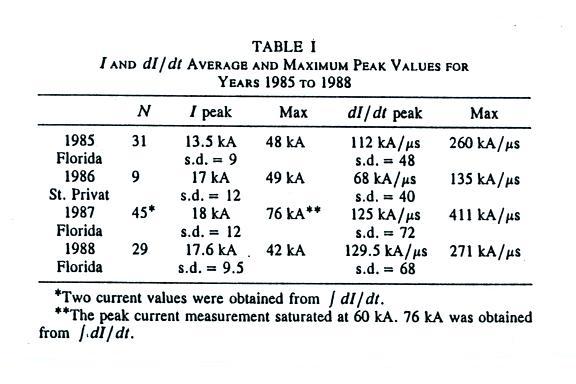
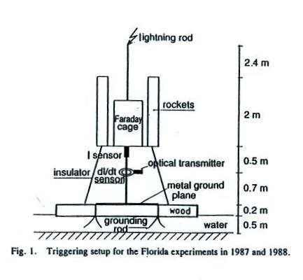
This first figure gives mean peak I and peak dI/dt values from rocket triggered lightning experiments conducted in Florida (at the Kennedy Space Center) and at the Saint Privat d'Allier station in central France (where the rocket triggered lightning experiments were first conducted).  With the exception of the 1986 St. Privat dI/dt data (where there appears to have been a shielding problem with the dI/dt sensor), the mean values from the different summer field experiments are generally in pretty good agreement.  The overall average peak I value is 16.6 kA and the average peak dI/dt value (France 1986 data omitted) is 122 kA/μs.  Remember that return strokes in triggered lightning are thought to be comparable to subsequent return strokes in natural lightning. 

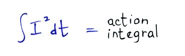
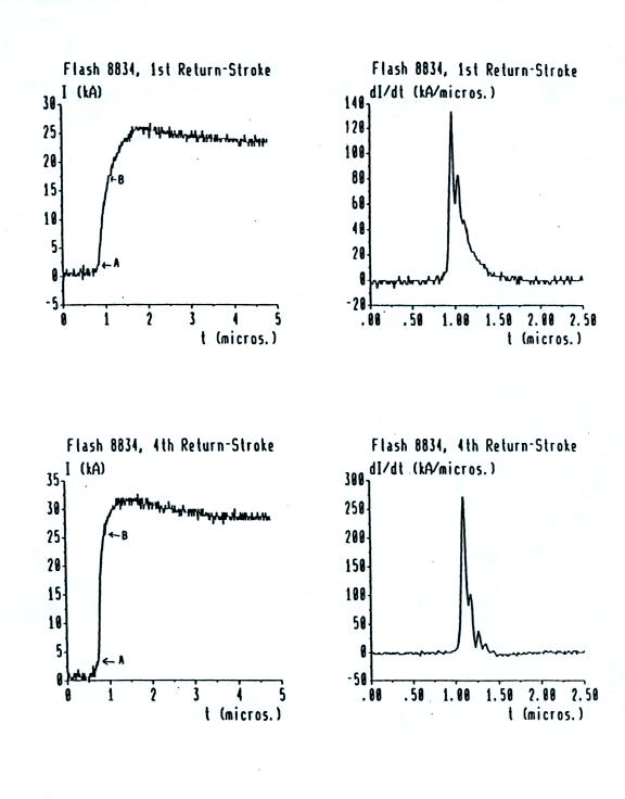
Lightning current parameters such as peak I and peak dI/dt are often log-normally distributed.  Data that are log-normally distributed should fall in a straight line on a cumlulative probability plot.  Cumulative probability distributions of peak I and peak dI/dt from the Florida 1987 and 1998 experiments are shown below.

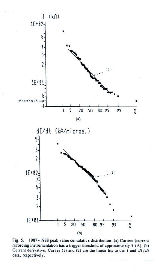
Parameters from these distributions are summarized in the table below together with parameters from the Swiss and Italian tower measurements.

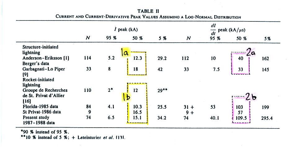
Generally the 50% values (the median) of peak I from the tower measurements (1a) compare very well with the peak I values from the rocket triggered lightning experiments (1b). 

The sensors and recording equipment used for the tower measurements in Switzerland and Italy probably didn't have fast enough time resolution to accurately measure peak dI/dt values.  The data in the table above seem to reflect this.  The tower derived measurements (2a): 40 and 33 kA/μs are significantly lower than the values obtained during the triggered lightning experiments (2b): 103 and 109.5 kA/μs. We should probably disregard the 57 kA/μs value from the St. Privat 1986 campaign.


Selected References

1.
  McEachron, K.B., "Lightning to the Empire State Building," J. Franklin Inst., 227, 149-217, 1939.

2.  Berger, K., "Novel Observations on Lightning Discharges: Results of Research on Mount San Salvatore," J. Franklin Inst., 283, 478-525, 1968.

3.  Berger, K., R.B. Anderson, and H. Kroninger, "Parameters of Lightning Flashes," Electra, No. 41, 23-37, 1975.

4.  Anderson, R.B., and A.J. Eriksson, "Lightning Parameters for Engineering Application," Electra, No. 69, 65-105, 1980.

5.  Garbagnati, E., F. Marinoni, G.B. LoPiparo, "Parameters of Lightning Currents.  Interpretation of the Results Obtained in Italy," 16th Intl. Conf. on Lightning Protection, Szeged, Hungary, 1981.


6.  Hussein, A.M., W. Janischewskyj, J.-S. Chang, V. Shostak, W.A. Chisolm, P. Dzurevych, and Z.-I. Kawasaki,"Simultaneous Measurement of Lightning Parameters for Strokes to the Toronto Canadian National Tower,"  J. Geophys. Res., 100, 8853-8861, 1995.

7. 
Leteinturier, C., J. Hamelin, and A. Eybert-Berard, "Submicrosecond Characteristics of Lightning Return-Stroke Currents,"  IEEE Trans. EMC., 33, 351-357, 1991.

8.  Fisher, R.J., G.H. Schnetzer, R. Thottappillil, V.A. Rakov, M.A. Uman, and J.D. Goldberg, "Parameters of Triggered-Lightning Flashes in Florida and Alabama,"  J. Geophys. Res., 98, 22887-22902, 1993.

Again, the links above will take you online e-journal copies (usually PDF files) of the article that I have accessed via the UA Library; they may not be available to you if you try from an off-campus computer.