Up to this point our study of thunderstorm electrical activity has concentrated mainly on the electric fields and E field changes recorded on the ground near thunderclouds.  We have also looked at some of the electrification processes that produce charge and at the distribution of charge inside the cloud.  Screening layers that form at the edges of electrified clouds make it difficult to determine the true amount and distribution of charge inside the cloud but we can use field change measurements to estimate amounts and locations of charge neutralized by lightning.


Today we will look at thunderstorms in a different way, as a quasi-steady current source.  We will look at how measurements of "Maxwell current" at the ground (Jm in the figure above) might allow us to make a reasonable lower limit estimate of the amplitude of the cloud current source.  We will also see that the Maxwell current varies relatively slowly during a storm which suggests that cloud electrification probably depends more on storm structure and storm dynamics than the cloud electric field.


We can start with the continuity equation and derive an expression for the Maxwell current:


The term in parentheses appears in one of Maxwell's equations - that is the origin of the name Maxwell current


A vector field with zero divergence is solenoidal and the vector field lines must form closed loops (see Example 2.7.2 in this online reference).  The following figure depicts the lines of Jm surrounding a current source in a thunderstorm (the current source is highlighted yellow).


We will first look at how you might measure Jm at a point (or at multiple points) on the ground.  With measurements at multiple points it might be possible to produce a surface map with contours of Jm (green in the figure above).  An area integration of
Jm might then provide an estimate of the strength of the current source in the cloud.  Note however that, because some of the lines of Jm do not reach the ground (shaded pink in the figure), an area integration will provide a lower limit estimate of the current source strength.

The figure above looks simple enough.  Once we start to see what Jm includes, however, it becomes a little harder (for me at least) to visualize field lines of Jm .


In the figure above we can see that
Jm includes lightning currents, JL, and field dependent conduction currents, JE.  There is a linear contribution to JE due to the drift of small ions in an electric field (conductivity times E field) and a non-linear component (corona discharge) that occurs when fields at the tips of sharp pointed objects on the ground exceed a certain threshold and corona starts to "spray" charge into the air.  Charged precipitation and transport of charge by wind motions are included in a convection current term, Jc.  Finally there is the displacement current term.


How do we determine Jm  at the ground?
1. You can measure it directly.  The figure below shows what a
"Jm sensor" might look like.

You basically dig up a piece of sod about 1 meter square, place it in a metal pan, and isolate the pan from ground.  Currents flowing to or from the test patch of soil (green) pass through an operational amplifier which converts the small amplitude currents into a measureable voltage.  The pan and the measuring electronics are positioned in a hole so that the top of the isolated soil is flush with the surroundings (the surroundings are brown in the figure above).  Note that the op-amp will keep the potential of the test pan at ground. 

The figure below shows an example of simultaneous records of E field and Maxwell current.


In the top figure you see 3 or 4 minutes of simultaneous recording of
Jm (top trace) and E field (bottom trace).  A portion of the record is shown on a faster time scale in the lower portion of the figure (Jm is the lower trace in this case).  Note that apart from the transient signals that occur during lightning discharges, Jm is fairly steady with time in these recordings (the green line).  In the top example the amplitude of  Jm does decrease slowly from about 10 nA/m2 at the start of the interval to about 7 nA/m2 at the end of the interval.

One important conclusion drawn from a plot like this is that, because Jm  remains relatively constant even when there are large changes in E field amplitude and polarity, the cloud electrication process must be independent of the E field.

2.    There may be situations where Jm is dominated by the displacement current term.  In that case you can determine Jm from E field recordings.  We'll write down the expression for Jm   again.

We'll determine Jm at a time when E is about zero (when E crosses zero following a lightning discharge as shown below). 


Then the field dependent conduction term will be zero.  We'll determine
Jm in between lightning discharges so that we won't have to include a lightning current term.  And we'll assume (for the time being anyway) that the convection current term is much smaller than the displacement current.


When all these conditions are true we'll be able to approximate
Jm by computing the displacement current.

The next figure gives us some idea how well this approach works:

The top curve (highlighted yellow) shows direct measurements of  Jm  made using the Jm sensor (the soil-filled pan) described in (1) above.  The blue shaded curve is an estimate of Jm made using measurements of the displacement current term (at times when E is zero) using field measurements made at the same site as the Jm sensor.  For the pink curve, measurements of the displacement current were made using field mills at nearby sites (field mills in the Kennedy Space Center network).  Estimates  of Jm could be made using measurements of displacement current at field mill sites east and west of the sensor site for example.  The value of Jm at the Jm sensor site could then be made by interpolating between the two nearby sites.  Lightning activity (number of discharges per 5 minute period) is plotted in the histogram at the bottom of the figure (shaded green).

The direct measurements of  are consistently 15% to 20% higher than the estimates derived from measurements of the displacement current.  The authors of the study state "this discrepancy is not large and probably due to a systematic error in the absolute calibration of the different sensors".


Next we'll look at one of the first attempts to map out values of
Jm over a large area.  The assumption is that Jm is dominated by the displacement current term.  Estimates of Jm were then made at multiple sites by measuring dE/dt at field mill sites in the KSC network.  The figure below shows an example of fields recorded at 6 of the sites .


A cloud-to-ground discharge was observed striking the ground at 16:57:23 and produced the field change near the start of each record.  A vertical arrow indicates where E crossed zero on each waveform.  This is the time at which dE/dt is measured and the displacement current term is computed.  The discharge at 16:58:39 (near the end of each record) was apparently an intracloud discharge.


The next figure is a contour map of E field change values for the 16:57:23 cloud-to-ground discharge. 

The field change values were computed after locating the charge neutralized during the CG flash using the chi-squared minimization procedure discussed in Lecture 12.  Approximately 46 C of negative charge located at an altitude of 8.1 km was neutralized during the flash.  The preceding figure and the figure to come are also from the reference cited in this figure.

The next figure shows contours of 
Jm determined just after the 16:57:23 CG flash (i.e. at the time E was crossing zero).


Note that the center of the
Jm pattern is near the center of the field change pattern.  The units of Jm  in the figure above are nA/m2.  An integration of Jm over area will provide an estimate of the strength of the current source in the cloud.  The next figure shows just such an estimate.

The two peaks in the plot of total current is explained by the fact that there were two storms cells active over the KSC field network during the time these data were collected.  Note the very reasonable (lower limit) estimate of 0.45 A peak total current.  Again the green-shaded histogram at the bottom of the figure shows lightning activity (number of discharges per 5 minute period).

Let's look at one more surprising result that can be obtained from estimates of Jm and displacement current.


We'll look at the field recovery following a lightning discharge and estimate
Jm at time to (when E crosses zero) and a time t that can be before or after to (i.e. it could be t1, t2, or t3 in the figure above). Jm at both to and t are shown above.  Now since Jm is relatively steady we can set Jm at times to and t equal to each other.

This leads to


Now we'll solve this expression for
JE(t)


It would be hard to determine or measure the convection terms so we try to find a way to eliminate them.  We're left with a way of estimating the conduction current term at times during the field recovery following a lightning flash. 


Since t in the equation could be
t1, t2, or t3, we have several estimates of JE and each is associated with a different value of E.


To clarify this point, to estimate JE(t1) you would compute dE/dt at to and t1 and use the formula above.  JE(t1) would be associated with E1.  We'd repeat the process using
to and t2, JE(t2) would be associated with E2.  If you plot all these pairs of JE and E on a graph you find they fall in a straight line.


You have a linear relationship between J and E.  The slope of the straight line is conductivity.  It appears that we have a means of estimating the air's conductivity.

Here's an example using actual data

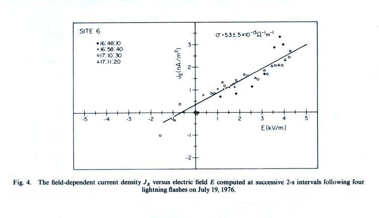
Estimates of conductivity ranged from 2 to 6 x 10-13 mhos/m.  Actual measurements of conductivity ranged from 0.4 to 1.8 x 10⁻¹⁴ mhos/m.  The agreement is not very good.  This idea didn't quite pan out.  The researchers that 
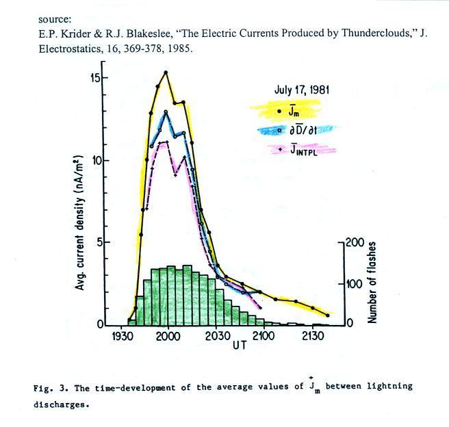
conducted the experiment concluded the estimates of conductivity "will be 
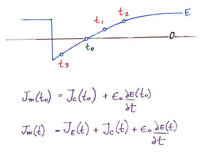
extremely sensitive to small time variations in the local Maxwell current density and must be modified to include these terms".