
Other than the high incidence of
positive CG discharge, E field soundings in thunderstorms have provided
evidence of the inverted charge structure. This is discussed in a
fairly recent paper that you can find here.
The
two
figures
below (on a class handout) illustrate E field soundings
in "normal" clouds and in clouds with inverted charge distributions.

Follow up studies seem to indicate that the graupel-ice crystal collision, non-inductive electrication mechanism that we have been studying is cable of explaining clouds with inverted charge distributions. This is shown on the figure below

Follow up studies seem to indicate that the graupel-ice crystal collision, non-inductive electrication mechanism that we have been studying is cable of explaining clouds with inverted charge distributions. This is shown on the figure below
In the center of the figure is the
graph that we examined in some detail last Thursday. It shows the
polarity of charge acquired by a graupel particle colliding with ice
crystals in a laboratory simulation of a cloud environment containing
supercooled water
droplets. The liquid water content on the vertical axis is a
measure of the supercooled droplet concentration.
Liquid water content in a typical cloud would be found near the level of the lower dotted line on the graph. The tripolar cloud charge distribution in a typical cloud is shown at left. High in the cloud where the temperature is cold, the graupel particle acquires negative charge and the ice crystals positive charge (region B on the graph). The ice crystals are carried upward and form the main positive charge center. The heavier graupel particle descends to form the main negative charge center. Somewhat lower in the cloud where temperatures are warmer than TR (a reversal temperature) but still below freezing the polarity of the charging changes (region C on the graph). The graupel ends up with positive charge and the ice crystals with negative charge. The positively charged graupel form the lower positive charge centers.
It seems that the unusual Central Plains storms have very high liquid water contents. If we look at the level of the upper dotted line on the charging graph in the center of the figure we see that the graupel particle always ends up with positive charge in this high LWC environment. There is no charge reversal temperature. The Reynolds, Brook, Gourley mechanism can explain clouds with inverted charge distributions.
The figure below was included on a class handout just to indicate that some very complex cloud charge distributions are found in the stratiform regions of Mesoscale Convective System (MCS) clouds (we didn't and won't spend anytime discussing the structure and formation of MCS clouds)
The main topic of the day was
looking a how we can use E field measurements at the ground to learn
about the location and amounts of charge involved in lightning
discharges. Most of the figures below were on handouts
distributed in class.
The data and results that we will be discussing come largely from experiments conducted at the Kennedy Space Center (KSC). A large network of electric field mills has been installed and is operating at KSC to identify and warn of thunderstorm and lightning hazards. The pre-1995 configuration of the field mill network is shown in the figure below (the network was upgraded in 1995).

The network that was operating up to 1995 has 0.1 second time
resolution. That is fast enough to resolve a lightning flash, but
not the individual return strokes that make up cloud to ground
flashes. The dynamic range was -15 kV/m to +15 kV/m and E field
signals were digitized with 30 V/m accuracy. The overall accuracy
of an individual field mill was about 10%.
The data and results that we will be discussing come largely from experiments conducted at the Kennedy Space Center (KSC). A large network of electric field mills has been installed and is operating at KSC to identify and warn of thunderstorm and lightning hazards. The pre-1995 configuration of the field mill network is shown in the figure below (the network was upgraded in 1995).
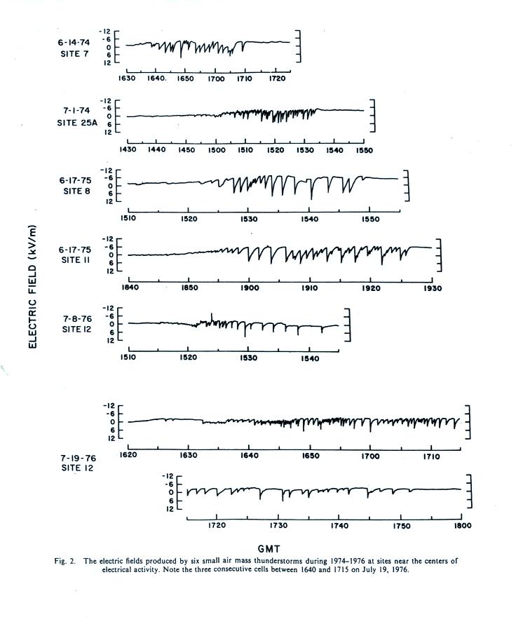
Examples of fields recorded during
6 small storms. Storms in this category lasted from 35 up to 85
minutes. Individual storms produced 16 to 82 discharges.
The maximum flashing rate during a small storm is 1 flash/minute.
A single example of a large storm E field record is shown below

A single example of a large storm E field record is shown below
Storms like this are often broken
into initial, very active, and end-of-storm-oscillation portions.
Note the very slow but large amplitude oscillations in the final EOSO
portion.
Large storms in the Livingston and Krider study had durations ranging from 75 to 265 minutes, produced 515 to 1212 discharges, and maintained flashing rates of 5 to 10 flashes per minute for 50 to 90 minutes. Number of flashes per 5 minute interval in a reprsentative large storm are shown in the histogram below.


Large storms in the Livingston and Krider study had durations ranging from 75 to 265 minutes, produced 515 to 1212 discharges, and maintained flashing rates of 5 to 10 flashes per minute for 50 to 90 minutes. Number of flashes per 5 minute interval in a reprsentative large storm are shown in the histogram below.
Fields at the ground are usually
lower than fields measured just a
few hundred meters above the ground. Space charge from corona
discharge at the ground limits the amplitudes of fields at the ground
and affects the shape of the field recovery between flashes. You
can get an accurate measurement of the field change at the ground (it
occurs so quickly that space charge can't be created or move quickly
enough to affect the field change value)

Measured field change values as a
function of distance. Note that small field change values are
sometimes observed very close to a discharge. This observation
will come up later in today's notes.
Now we will begin to look at what you can do with simultaneous measurements of field change values at multiple field mill sites.

We'll consider the simplest model of a cloud-to-ground discharge and assume that the charge neutralized by the flash comes from a uniform sphere of charge in the cloud. You can treat this as a single point charge (Point 1). We will try to use the delta E measurements to determine the location (x, y, and z coordinates) and magntitude of the neutralized charge (delta Q).
We show the location of one of the field mill sites in the figure. At that location we will have a measurement of the field change. We can also calculate the field change that the charge neutralized at Point 1 would produce; the expression for this calculated field change is shown at Point 2.
We have pairs of measured and calculated for all or most of the field mill sites. The idea then is to adjust x, y, z, and delta Q until the chi-squared function at Point 4 is minimized.

Some of the results obtained using the single charge model. Fig. 1 shows the magnitude of the charge neturalized. Fig. 2 shows that this charge was largely found between 6 and 9 or 10 km altitude, in the -10 to -35 C temperature range. Fig. 3 shows that 75% of cloud-to-ground discharges strike the ground at a distance, D, of 5 km (3 miles) or less from the center of the charge neutralized by the flash. 95% of the discharges strike the ground within 8 km (5 miles) of the charge center. The distance D is shown in the figure below.


Now we will begin to look at what you can do with simultaneous measurements of field change values at multiple field mill sites.
We'll consider the simplest model of a cloud-to-ground discharge and assume that the charge neutralized by the flash comes from a uniform sphere of charge in the cloud. You can treat this as a single point charge (Point 1). We will try to use the delta E measurements to determine the location (x, y, and z coordinates) and magntitude of the neutralized charge (delta Q).
We show the location of one of the field mill sites in the figure. At that location we will have a measurement of the field change. We can also calculate the field change that the charge neutralized at Point 1 would produce; the expression for this calculated field change is shown at Point 2.
We have pairs of measured and calculated for all or most of the field mill sites. The idea then is to adjust x, y, z, and delta Q until the chi-squared function at Point 4 is minimized.
Some of the results obtained using the single charge model. Fig. 1 shows the magnitude of the charge neturalized. Fig. 2 shows that this charge was largely found between 6 and 9 or 10 km altitude, in the -10 to -35 C temperature range. Fig. 3 shows that 75% of cloud-to-ground discharges strike the ground at a distance, D, of 5 km (3 miles) or less from the center of the charge neutralized by the flash. 95% of the discharges strike the ground within 8 km (5 miles) of the charge center. The distance D is shown in the figure below.
Instead of getting larger as you
get closer to the storms center,
field charges at the ground are often either very small or of opposite
polarity. This suggested that a lower volume of positive charge
might be involved in cloud-to-ground discharges. This led to the
development of a 2 charge model, illustrated below.

This is the most general form of
the two charge model. The two charges can have different
magnitudes and can have completely different locations in space ( the
point dipole model assumes the two charges are of equal amplitude but
opposite polarity, another model assumes the two charges are aligned
vertically. The calculated field change expression now contains 8
unknowns.
The next two figures shows some of the results obtained with this arbitrary 2 charge model.

The next two figures shows some of the results obtained with this arbitrary 2 charge model.
The circles indicate charge
neutralized during lightning discharges. Cross hatched circles
are positive, open circle negative charge. The radius of the
circle gives you an idea of the amount of charge neutralized.
Both intracloud and cloud to ground discharges are plotted. An example of each is shown. Intracloud discharges involve positive charge in the main positive charge center located in the upper portion of the thundercloud and negative charge in the main negative charge center in the middle of the cloud. Cloud-to-ground discharges seem to almost always involve negative charge in the middle of the cloud and positive charge in one of the lower positive charge centers.
The next figure is from a little more active thunderstorm cell.

Note the tendency for the altitudes of the positive charges neutralized in intracloud discharges to be found at higher altitude toward the middle and perhaps the end of the storm. Also the amounts of charge neutralized in discharges appears to increase with time (larger diameter circles toward the end of the storm).
The chi-squared procedure for determining charge center locations and charge magnitudes using multi-station field change measurements has also be used with Slow E field antenna systems. Slow E records have faster time resolution and can faithfully record the field changes produced by the separate return strokes in a cloud to ground flash.
A description of an 8-station slow E antenna and an example of a CG flash slow E field record (containing 5 or 6 return strokes) is shown in the figure below (on a class handout).

The network was installed near Socorro New Mexico and operated by the New Mexico Institute of Mining and Technology (I was an undergraduate student there). The figure below shows locations of the charges neutralized by the separate return stroke in 4 cloud-to-ground flashes. The simple point charge model was assumed.

Both intracloud and cloud to ground discharges are plotted. An example of each is shown. Intracloud discharges involve positive charge in the main positive charge center located in the upper portion of the thundercloud and negative charge in the main negative charge center in the middle of the cloud. Cloud-to-ground discharges seem to almost always involve negative charge in the middle of the cloud and positive charge in one of the lower positive charge centers.
The next figure is from a little more active thunderstorm cell.
Note the tendency for the altitudes of the positive charges neutralized in intracloud discharges to be found at higher altitude toward the middle and perhaps the end of the storm. Also the amounts of charge neutralized in discharges appears to increase with time (larger diameter circles toward the end of the storm).
The chi-squared procedure for determining charge center locations and charge magnitudes using multi-station field change measurements has also be used with Slow E field antenna systems. Slow E records have faster time resolution and can faithfully record the field changes produced by the separate return strokes in a cloud to ground flash.
A description of an 8-station slow E antenna and an example of a CG flash slow E field record (containing 5 or 6 return strokes) is shown in the figure below (on a class handout).
The network was installed near Socorro New Mexico and operated by the New Mexico Institute of Mining and Technology (I was an undergraduate student there). The figure below shows locations of the charges neutralized by the separate return stroke in 4 cloud-to-ground flashes. The simple point charge model was assumed.
Notice that each of the return
strokes "taps" charge from a slightly different location in the cloud.