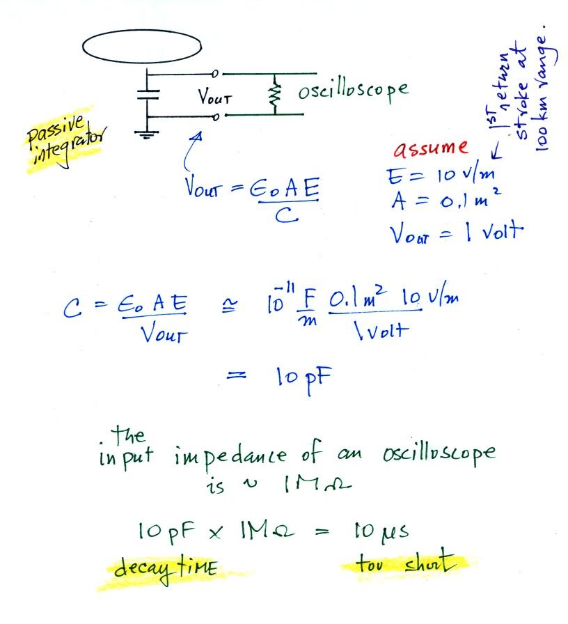
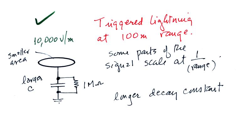
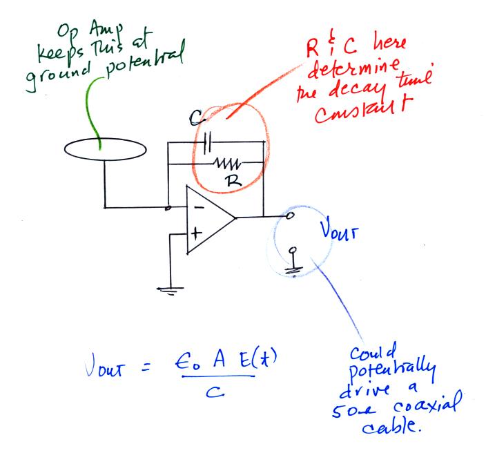
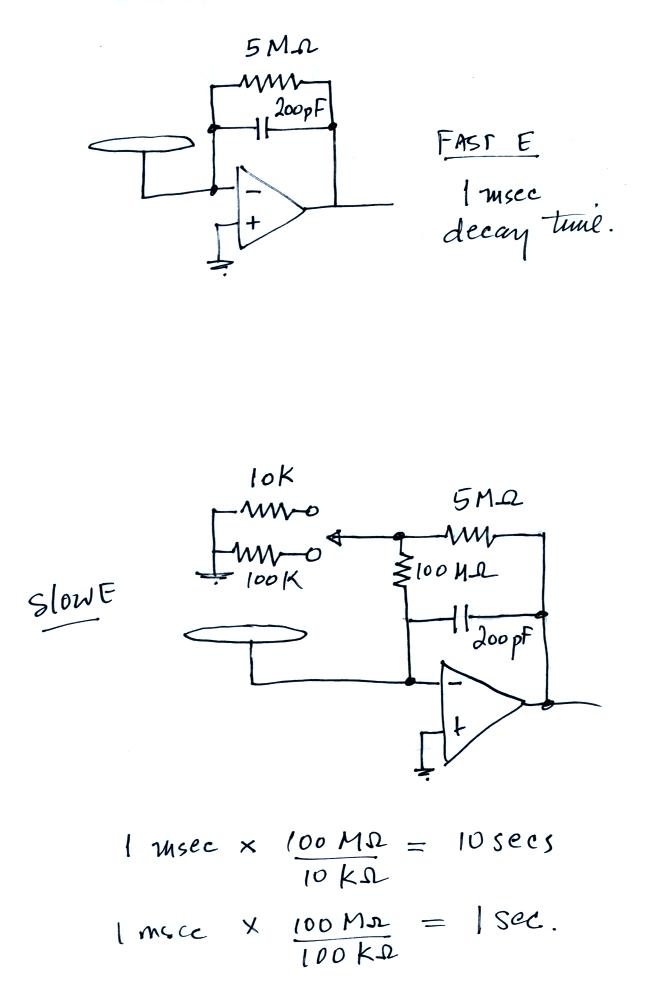
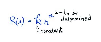
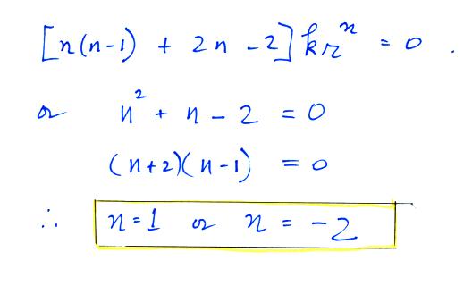
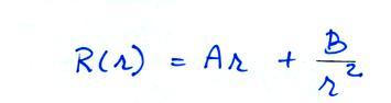
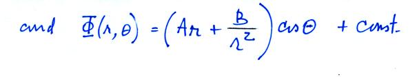
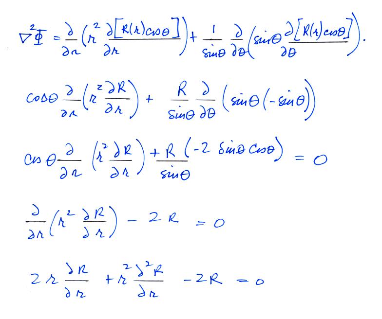
.
Enhancement
of
fields
by conducting objects is an important
concern. In some cases (we'll look
at an example or two later) the enhanced
field is strong enough to initiate or
trigger a lightning discharge.
The following handout gives a rough,
back-of-the-envelope kind of estimate of
the factor of enhancement.
This might
require a little explanation.
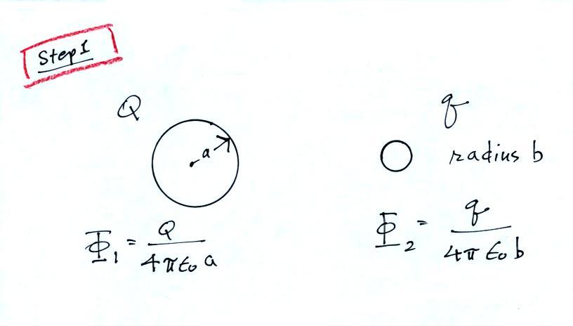
First you
write down the potential at the surface of
two conducting spheres of radius a and b,
carrying charges Q and q (really just the
potential a distance a or b from a point
charge Q or q)
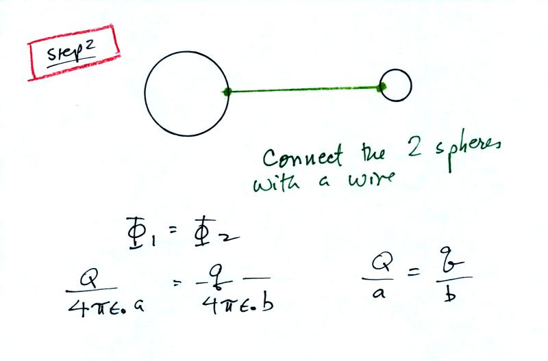
Then you
connect the two spheres with a wire which
forces the two potentials to be equal
(this would of course cause the charge to
rearrange themselves and turn this into a
much more complex problem, but we will
ignore that).
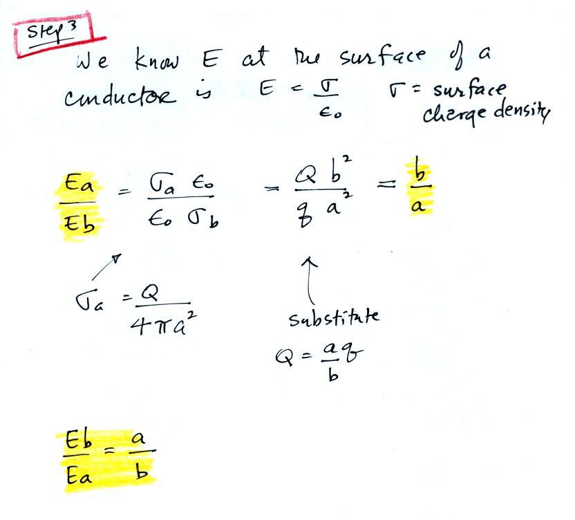
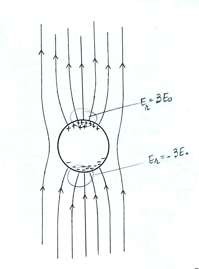
Finally we
write down expressions for the relative
strengths of the electric fields at the
surfaces of the two spheres (we assume Q
and q would be uniformly spread out over
the two spheres which wouldn't be
true). We see that the field at the
surface of the smaller sphere is a/b times
larger than the field at the surface of
the bigger sphere.
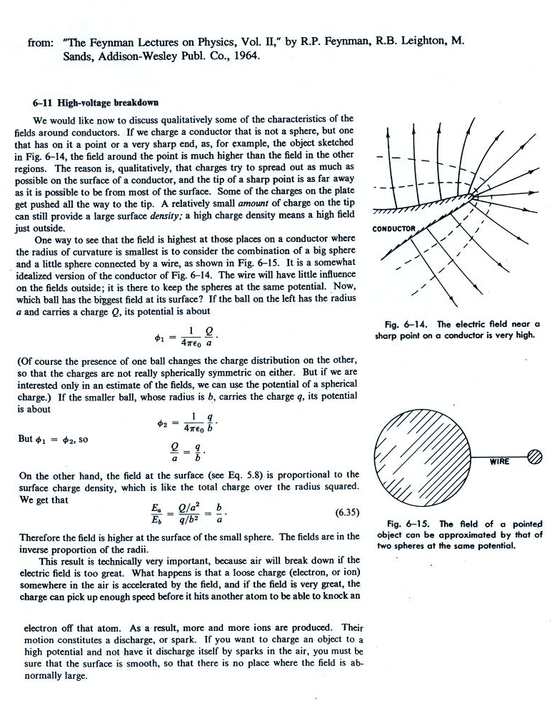
Here is a real example
of field enhancement that lead to
triggering of a lightning strike and
subsequent loss of a launch vehicle
(you'll find the entire article here)
In this case the
rocket body together with the exhaust
plume created a long pointed conducting
object. Enhanced fields at the top
and bottom triggered lightning.
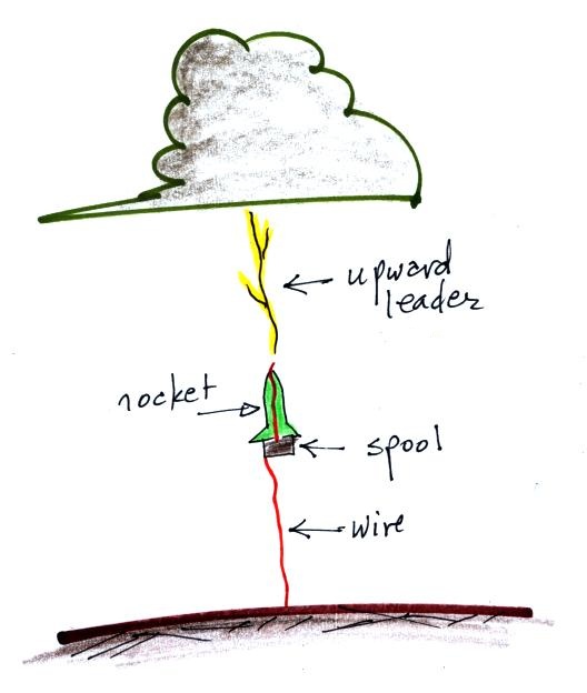
We'll talk about
triggered lightning later in the
course. I'm referring to lightning
that is purposely trigger so that it can
strike instrumentation on the ground and
studied at close range.
The basic idea is to launch a small
rocket (about 3 feet tall) in a high
electric field under a thunderstorm.
A spool of wire is mounted on the tail
fins of the rocket. One end of the
wire is connected to ground and the other
end runs up to the nose of the
rocket. Wire un-spools (probably the
hardest part is to keep the wire from
breaking) once the rocket is launched
forming a narrow tall conducting
object. Field enhancement at the top
of the rocket is enough often times to
initiate an upward leader discharge that
then triggers lightning.
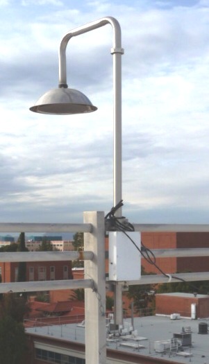
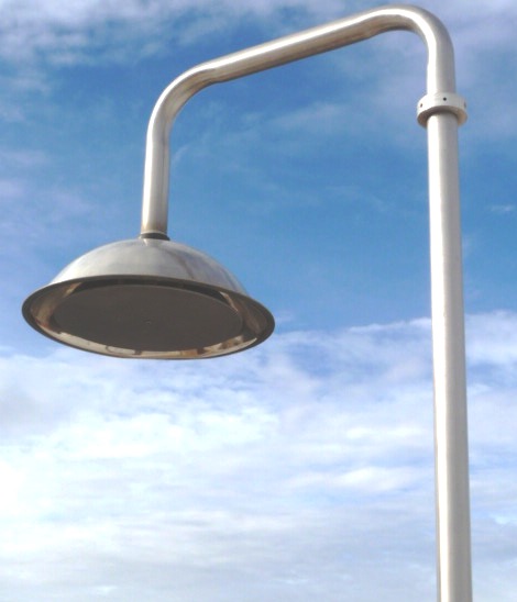
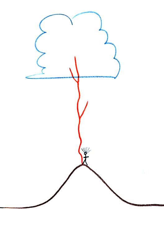
Enhancement of the E field
at the top of a mountain (or tall building
or structure) is sometimes high enough to
trigger lightning also.
Note the direction of
the branching. This indicates that
this discharge began with a leader process
that traveled upward from the
mountain. Most cloud to ground
lightning discharges begin with a leader
that propagates from the cloud downward
toward the ground. We will of course
look at the events that occur during
lightning discharges in a lot more detail
later in the semester.
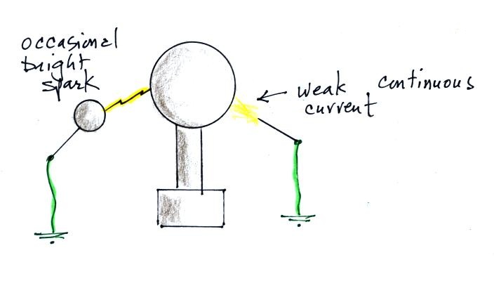
And finally (will this lecture ever
end). The ability of a point to draw
off or throw off electrical charged that
so interested Benjamin Franklin involves
enhancement of the E field.
A pointed conductor brought near a Van
de Graaff generator enhances the field
enough to ionize air and create charge
carries in the air. A weak current
flows between the Van de Graaff and the
point. Charge on the generator is
not able to build to the point where a
large bright spark occurs.