Because CO2 is an important greenhouse gas and the greenhouse effect warms the earth, the obvious question is what has the temperature of the earth been doing during this period? In particular has the earth warmed since the mid 1700s?
We will address this question about temperature in two parts.
1. Direct measurements of temperature
People have been making accurate measurements of temperature (on land and at sea) at a multitude of locations around the globe for the past 150 years or so. The sketch below gives you a rough idea of what these data show (global temperature values are shown on the vertical scale on the right side of the figure, the scale on the left compares the global average temperature at a particular time with the 1961-1990 mean).
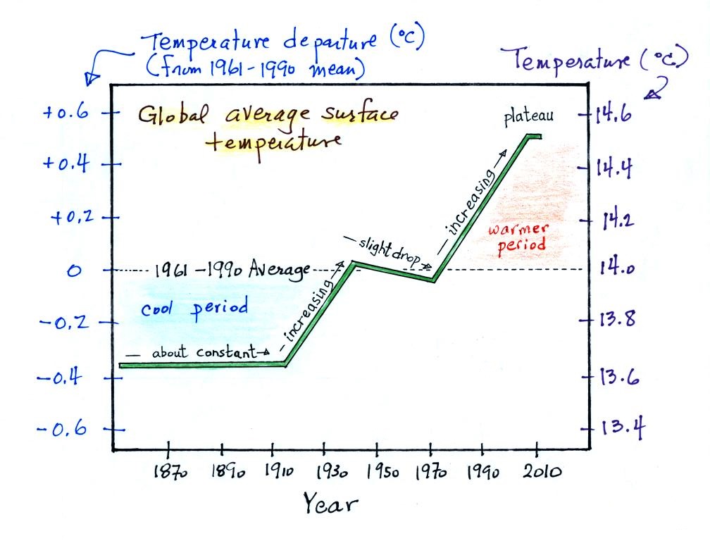
Overall temperature appears to have increased about 0.8o C during this period. We can get some feel for how significant a 1oC change in global average temperature is by looking back perhaps 20,000 years when the earth was in the middle of a glacial period (often referred to as an ice age). At that time global average temperature was about 5o C cooler than at present and a large thick sheet of ice, the Laurentide Ice Sheet, covered most of Canada and a sizable portion of the northern United States.
Detecting a small but significant change in global average temperature is not easy to do. There is a lot of natural variation from year to year that masks longer term changes. The large year to year variations have been left out of the figure above so that the overall trend could be seen more clearly. The figure below does show the year to year variation (black line with dots) and the uncertainties (the green bars) in the yearly measurements (note how the uncertainty is lower in the more recent measurements).
Not only is there a lot of year to year variability, but the instruments used to measure temperature have changed a lot. The locations at which temperature measurements have been made have also changed (try to imagine how the city of Tucson might have looked 130 years ago). About 2/3rds of the earth's surface is ocean and measurements were few and far between during much of this time period (sea surface temperatures can now be measured using satellites).
These
data are from a NASA
Goddard Institute for Space Studies site.
The term "Temperature Anomaly" on the vertical axis means the temperatures for a particular year are compared with the mean temperature computed over a 30 year period from 1951-1980. Temperatures prior to about 1935 were colder than the 1951-1980 mean and temperatures after about 1975 were warmer.
Here's another independent determination of global temperature change over a slightly longer time period from the University of East Anglia Climatic Research Unit.
The
overall tendency seems to be the same
in both cases.
We should mention that the observed warming has not been uniformly distributed over the surface of the earth. Have a look at these data from the 2000-2009 period that show the that greatest warming has occurred in the Arctic.
2. Proxy estimates of temperature
The direct measurements of temperature (made with thermometers) extend back to the mid 1800s. It would be interesting to know how temperature was changing prior to that. This is similar to what happened when the scientists wanted to know what carbon dioxide concentrations looked like prior to 1958. In that case they were able to go back and analyze air samples from the past (air trapped in bubbles in ice sheets).
That doesn't work with temperature. To understand why, imagine putting some air in a bottle, sealing the bottle, putting the bottle on a shelf, and letting it sit for 100 years. After a century had elapsed you could take the bottle down from the shelf, carefully remove the air, and measure what the CO2 concentration in the air had been when the air was sealed in the bottle. You couldn't, on the other hand, use the air in the bottle to determine what the temperature of the air was when it was originally placed on the shelf.
With temperature (and other climate variables) you need to use proxy data. You need to look for something else whose presence, concentration, or composition depends on temperature.
Here's a proxy data
"example."
Let's say you want to determine how many students are living in a house near a university.

We should mention that the observed warming has not been uniformly distributed over the surface of the earth. Have a look at these data from the 2000-2009 period that show the that greatest warming has occurred in the Arctic.
2. Proxy estimates of temperature
The direct measurements of temperature (made with thermometers) extend back to the mid 1800s. It would be interesting to know how temperature was changing prior to that. This is similar to what happened when the scientists wanted to know what carbon dioxide concentrations looked like prior to 1958. In that case they were able to go back and analyze air samples from the past (air trapped in bubbles in ice sheets).
That doesn't work with temperature. To understand why, imagine putting some air in a bottle, sealing the bottle, putting the bottle on a shelf, and letting it sit for 100 years. After a century had elapsed you could take the bottle down from the shelf, carefully remove the air, and measure what the CO2 concentration in the air had been when the air was sealed in the bottle. You couldn't, on the other hand, use the air in the bottle to determine what the temperature of the air was when it was originally placed on the shelf.
With temperature (and other climate variables) you need to use proxy data. You need to look for something else whose presence, concentration, or composition depends on temperature.
Let's say you want to determine how many students are living in a house near a university.
You
could
walk by the house late in the
afternoon, when the students might
be outside, and count them.
That would be a direct
measurement. There could still be
some errors in your measurement
(some students might be inside the
house and might not be counted,
some of the people outside might
not actually live at the house).
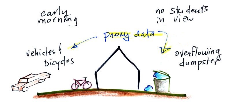
If you were to walk by early in the morning it is likely that the students would be inside sleeping. In that case you might look for other clues (such as the size of the house, or the number of automobiles or bicycles parked in the yard) that might give you an idea of how many students lived there. Some calibration would be needed but you could use this other information to estimate the number of students present.
3. Paleoclimatology
Scientists have come up with a variety of ingenious ways of determining past temperature and climate. Several of them are shown in the figure below. Pay careful attention to the logarithmic time scale at the bottom of the figure. It probably should have been labeled time before the present. The present day is shown at right and is marked zero.
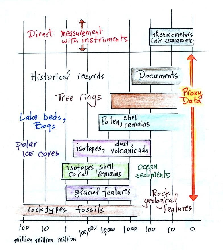
We'll work our way from the bottom to the top of the chart and briefly look at a few examples.
3a. Geological evidence
Earlier in the course we saw how the banded iron rock formation provides evidence of the early buildup of oxygen in the oceans. The oxygen was produced by blue-green algae using photosynthesis at a time (roughly 2 to 3 billion years ago) when there was little or no oxygen in the earth's atmosphere. We may also have mentioned red beds, sedimentary rock that has a rusty color because it contains iron oxides. These red beds are evidence of oxygen buildup in the atmosphere. The photograph below from Red Rock State Park near Sedona (in northern Arizona) shows Permian red beds (source of this image).
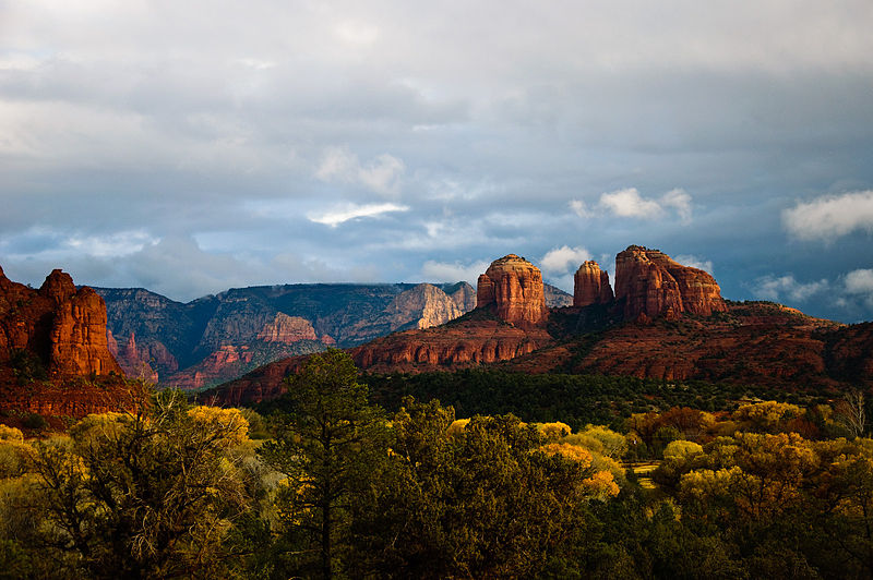
The Permian period was roughly 250 to 300 million years ago. There are red beds older than that but not more than 2 billion years old.
Rocks and geological formations can tell us a lot about the distant past. The earth has been alternating between glacial and interglacial periods for the past 1 to 2 million years (more about this in Part 3 of this series). Evidence of glacial periods is often preserved in rock.
U-shaped valleys with steep sides and a relatively flat bottoms are produced by the scouring action of glaciers moving downhill. The grinding motion of the ice against stone will often leave clearly visible striations.
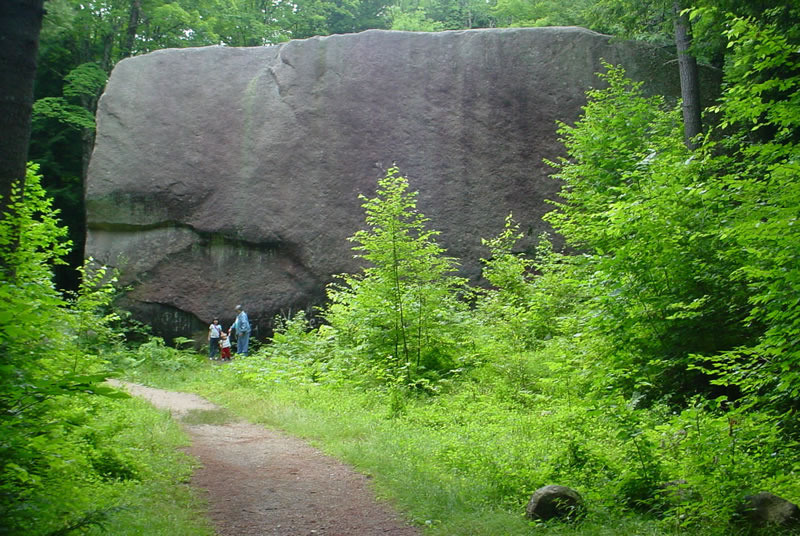
An erratic (also called a dropstone) is a large rock or boulder carried by a glacier and then dropped when the ice melted. Erratics are often found quite far from their place of origin and often in a region with completely different types of soil and rock.
The 12 million pound Madison Boulder shown above is the largest erratic in New England and one of the largest in the world. Plymouth Rock, near where the Mayflower landed in 1620, is apparently also a glacial erratic (it has been moved from its original location to a more protected site because of its historical significance). Dropstones can also be carried by icebergs and fall to the sea floor when the iceberg melts. Stones in Erratic Rock State Natural Site in Oregon were carried more than 500 miles during ice age flooding of the Columbia River.
Glaciers erode the surface over which they move and produce sediment, "till", that is an unsorted mix of many particle or rock sizes.
3b. Ocean and lake sediments
Life forms in ocean fall to the ocean floor when they die. Sea floor sediments build up year after year and are probably the longest continuous record of climate change that is available.
Plant pollen and spores are abundant and particularly well preserved in core samples from lake beds and the sea floor. With care they can be used to infer past environmental and climatic conditions. Size scales weren't included in the figures above, but the examples shown are probably 10 to a few 10s of micrometers (millionths of a meter) across. Identification (and dating) of the types of pollen present provides information about the environmental conditions at the time.
The photographs above are from an online article titled "Tropical rainforest on the South Pole" from Ultrecht University in the Netherlands.
3c. Tree rings
Tree rings (dendrochronology) provide another way of determine recent changes in climate.
The date of each ring can be determined. The widths of the rings are determined by temperature and precipitation during the year of that growth (and other factors). Bristlecone pine trees in the United States provide a continuous record of climate change that extends back about 8500 years. A record this long does not come, of course, from a single tree.
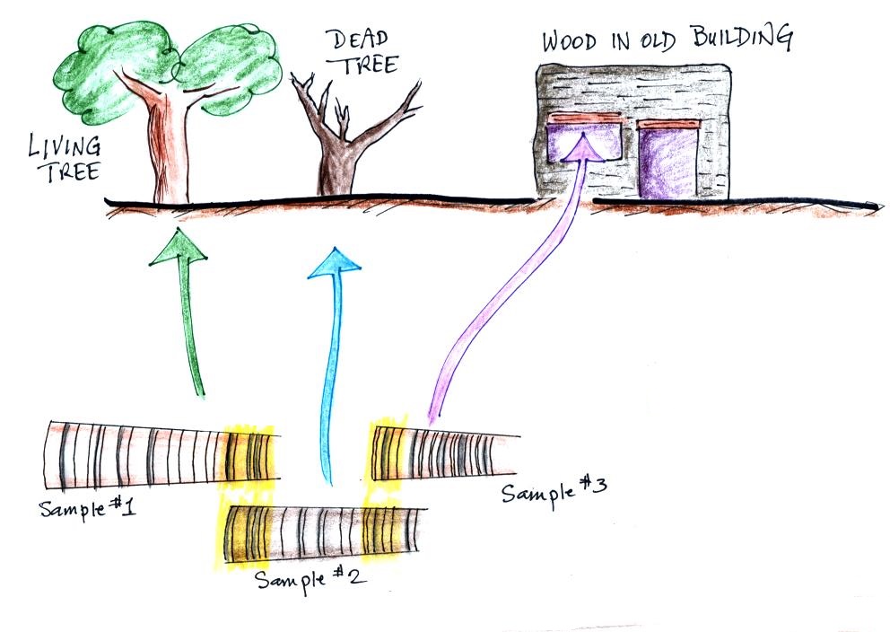
Rather part of the pattern of rings in a living tree can be matched to a portion of the of rings in an older, dead tree and used to date that tree. The dead tree record which now extends further back in time than the living tree can be used to date a third tree and so on further and further back in time. Or, as shown in the figure above, cross matching between several wood samples can be used to date the wood in an old structure of historical interest.
3d. Historical documents
Historical records such as time and types of crops that were planted and whether the ensuring harvest was good or bad; exceptional periods of cold or heat, droughts, snow or storm damage provide a qualitative idea of the climate at the time.
From written accounts of Norse sagas (and much later archaeological work) we know that Vikings settled Iceland, Greenland, and parts of Newfoundland during a warm period that lasted from about AD 800 to AD 1300. Iceland was apparently settled between about 874 AD and 930 AD. One of the early settlers, Erik the Red, was banished from Iceland (for manslaughter) and is credited with establishing the first colony on Greenland in about 985 AD. Settlements on Greenland lasted nearly 500 years, until the climate began to cool. The total population reached several 1000 people. Leif Erikson, the son of Erik the Red, is often credited with the establishment of the first Norse settlement on North America (at L'Anse aux Meadows in Newfoundland in about 1000 AD).
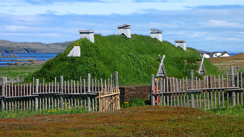
Recreation of a sod longhouse at L'Anse aux Meadows, Newfoundland (source of this image)
If you were to walk by early in the morning it is likely that the students would be inside sleeping. In that case you might look for other clues (such as the size of the house, or the number of automobiles or bicycles parked in the yard) that might give you an idea of how many students lived there. Some calibration would be needed but you could use this other information to estimate the number of students present.
3. Paleoclimatology
Scientists have come up with a variety of ingenious ways of determining past temperature and climate. Several of them are shown in the figure below. Pay careful attention to the logarithmic time scale at the bottom of the figure. It probably should have been labeled time before the present. The present day is shown at right and is marked zero.
We'll work our way from the bottom to the top of the chart and briefly look at a few examples.
3a. Geological evidence
Earlier in the course we saw how the banded iron rock formation provides evidence of the early buildup of oxygen in the oceans. The oxygen was produced by blue-green algae using photosynthesis at a time (roughly 2 to 3 billion years ago) when there was little or no oxygen in the earth's atmosphere. We may also have mentioned red beds, sedimentary rock that has a rusty color because it contains iron oxides. These red beds are evidence of oxygen buildup in the atmosphere. The photograph below from Red Rock State Park near Sedona (in northern Arizona) shows Permian red beds (source of this image).
The Permian period was roughly 250 to 300 million years ago. There are red beds older than that but not more than 2 billion years old.
Rocks and geological formations can tell us a lot about the distant past. The earth has been alternating between glacial and interglacial periods for the past 1 to 2 million years (more about this in Part 3 of this series). Evidence of glacial periods is often preserved in rock.
 |
 |
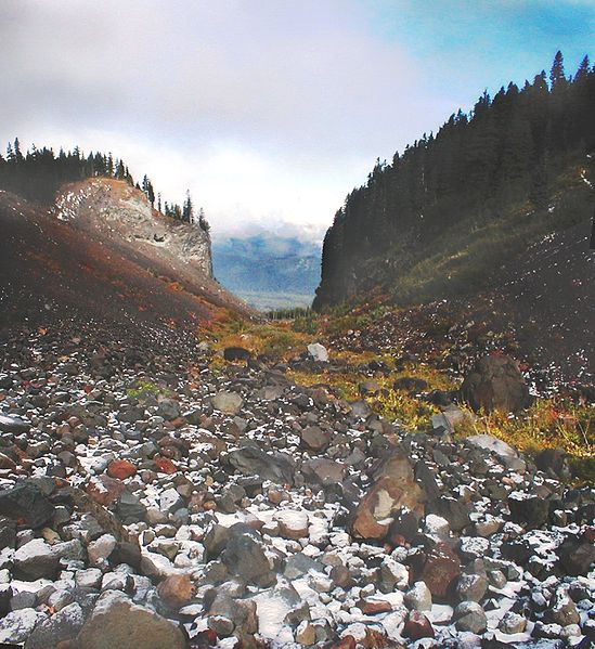
| A U-shaped valley
carved out by a relatively small
glacier in the Mt. Hood Wilderness (source of this
photograph) |
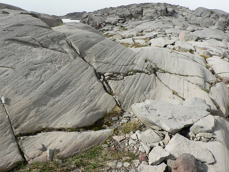
Glacial striations
found in the Mt. Rainier National
Park (source
of this image) |
U-shaped valleys with steep sides and a relatively flat bottoms are produced by the scouring action of glaciers moving downhill. The grinding motion of the ice against stone will often leave clearly visible striations.
 |
 |
| A photograph of the
Madison Boulder in New Hampshire
(from Atlas
Obscura). |
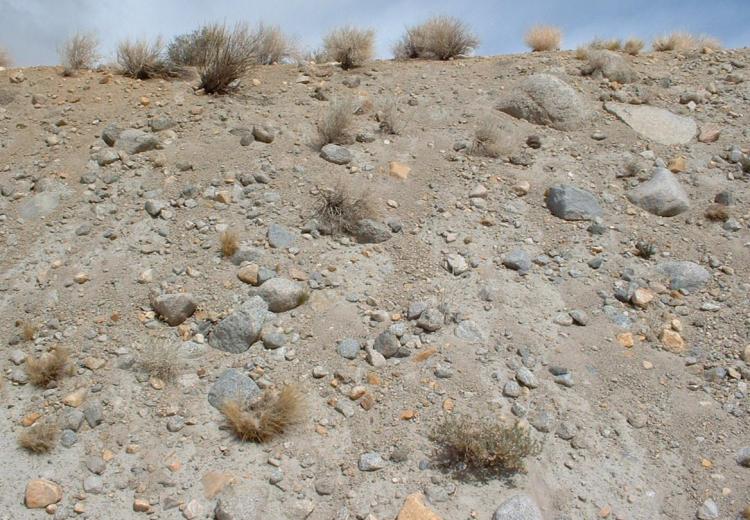
Glacial till
(produced and moved around by a
glacier) exposed in a road cut (source
of this photograph) |
An erratic (also called a dropstone) is a large rock or boulder carried by a glacier and then dropped when the ice melted. Erratics are often found quite far from their place of origin and often in a region with completely different types of soil and rock.
The 12 million pound Madison Boulder shown above is the largest erratic in New England and one of the largest in the world. Plymouth Rock, near where the Mayflower landed in 1620, is apparently also a glacial erratic (it has been moved from its original location to a more protected site because of its historical significance). Dropstones can also be carried by icebergs and fall to the sea floor when the iceberg melts. Stones in Erratic Rock State Natural Site in Oregon were carried more than 500 miles during ice age flooding of the Columbia River.
Glaciers erode the surface over which they move and produce sediment, "till", that is an unsorted mix of many particle or rock sizes.
3b. Ocean and lake sediments
Life forms in ocean fall to the ocean floor when they die. Sea floor sediments build up year after year and are probably the longest continuous record of climate change that is available.
 |
 |
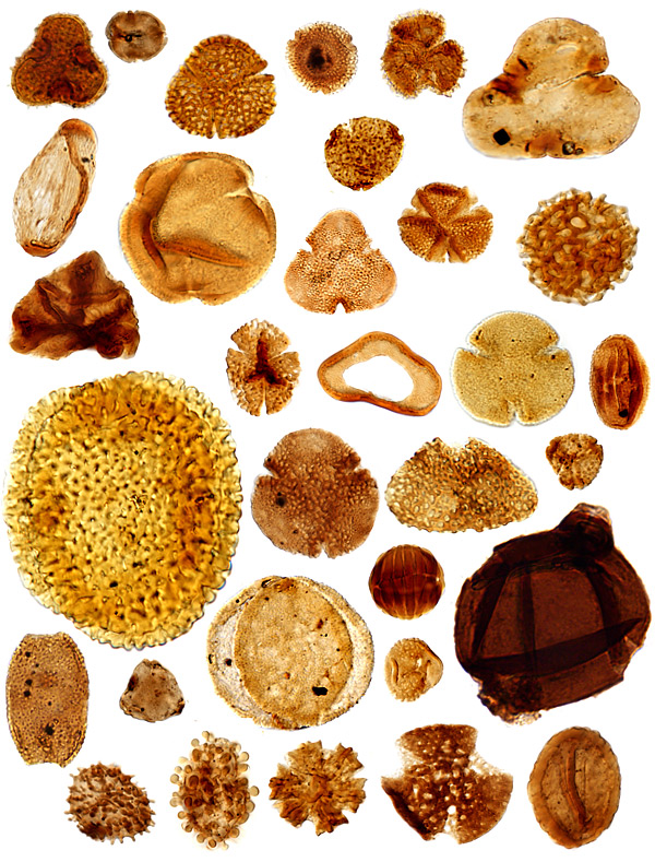 |
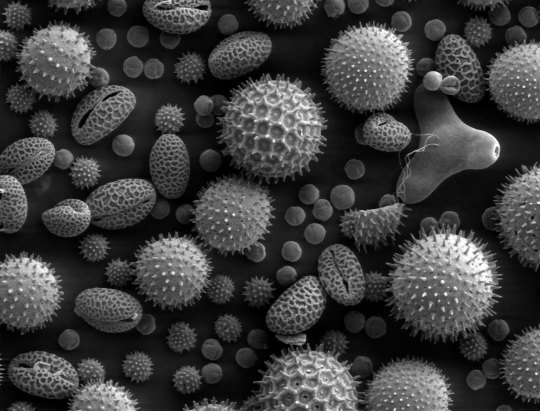
| Scanning electron
microscope photograph of grains of
(unfossilized) pollen. (source) |
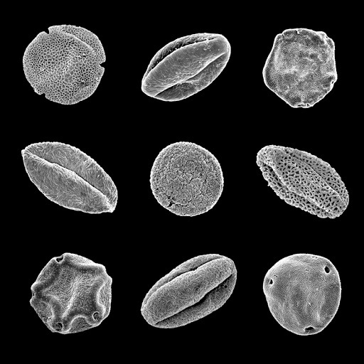
Fossilized pollen
from China. (source) |
Electron microscope
photographs of fossilized pollen
from the Paleocene-Eocene Thermal
Maximum 56.3 million years ago. (source) |
Plant pollen and spores are abundant and particularly well preserved in core samples from lake beds and the sea floor. With care they can be used to infer past environmental and climatic conditions. Size scales weren't included in the figures above, but the examples shown are probably 10 to a few 10s of micrometers (millionths of a meter) across. Identification (and dating) of the types of pollen present provides information about the environmental conditions at the time.
 |
 |
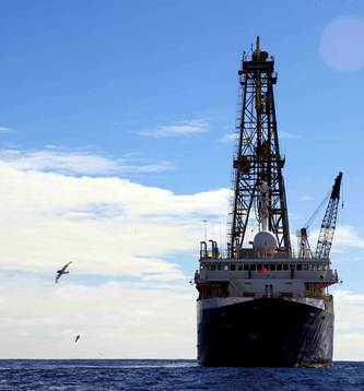
| The drill ship JOIDES
Resolution located off the
coast of Antarctica in Spring
2010. Researchers were able to
drill 1000 m below the sea floor and
obtained sediment samples that were
over 50 million years old.
(photo credit: Rob Dunbar Stanford
University |
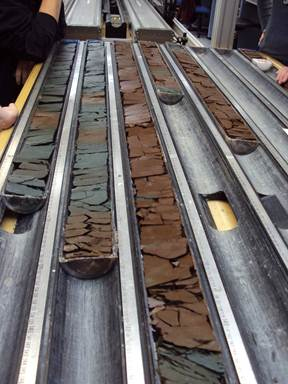
Photographs of core
samples obtained during the
expedition. Pollen and spores
were preserved in the marine
sediment. (photo credit: Kevin Welsh
University of Queensland) |
The photographs above are from an online article titled "Tropical rainforest on the South Pole" from Ultrecht University in the Netherlands.
3c. Tree rings
Tree rings (dendrochronology) provide another way of determine recent changes in climate.
 |
 |
| Tree rings form
because of changes in the rate of
growth of a tree during the
year. Light colored low
density wood forms early in the
year. A thinner, darker, more
dense band forms late in the
year. (source
of this image) |
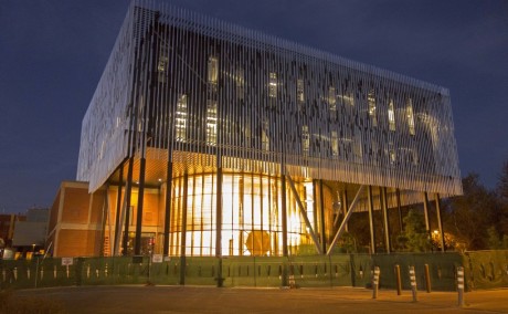
The Laboratory
of Tree Ring Research at the
University of Arizona recently moved
into this new building. Their
offices and laboratories used to be
located in the football stadium. |
The date of each ring can be determined. The widths of the rings are determined by temperature and precipitation during the year of that growth (and other factors). Bristlecone pine trees in the United States provide a continuous record of climate change that extends back about 8500 years. A record this long does not come, of course, from a single tree.
Rather part of the pattern of rings in a living tree can be matched to a portion of the of rings in an older, dead tree and used to date that tree. The dead tree record which now extends further back in time than the living tree can be used to date a third tree and so on further and further back in time. Or, as shown in the figure above, cross matching between several wood samples can be used to date the wood in an old structure of historical interest.
3d. Historical documents
Historical records such as time and types of crops that were planted and whether the ensuring harvest was good or bad; exceptional periods of cold or heat, droughts, snow or storm damage provide a qualitative idea of the climate at the time.
From written accounts of Norse sagas (and much later archaeological work) we know that Vikings settled Iceland, Greenland, and parts of Newfoundland during a warm period that lasted from about AD 800 to AD 1300. Iceland was apparently settled between about 874 AD and 930 AD. One of the early settlers, Erik the Red, was banished from Iceland (for manslaughter) and is credited with establishing the first colony on Greenland in about 985 AD. Settlements on Greenland lasted nearly 500 years, until the climate began to cool. The total population reached several 1000 people. Leif Erikson, the son of Erik the Red, is often credited with the establishment of the first Norse settlement on North America (at L'Anse aux Meadows in Newfoundland in about 1000 AD).
Recreation of a sod longhouse at L'Anse aux Meadows, Newfoundland (source of this image)
3e.
Isotopic analyses
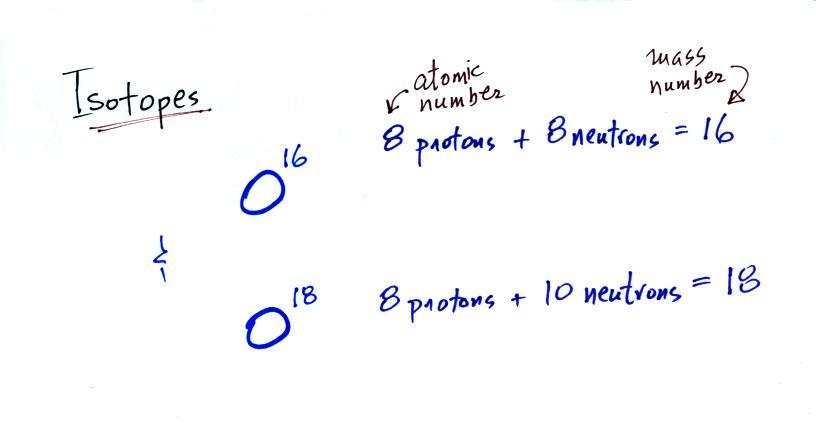
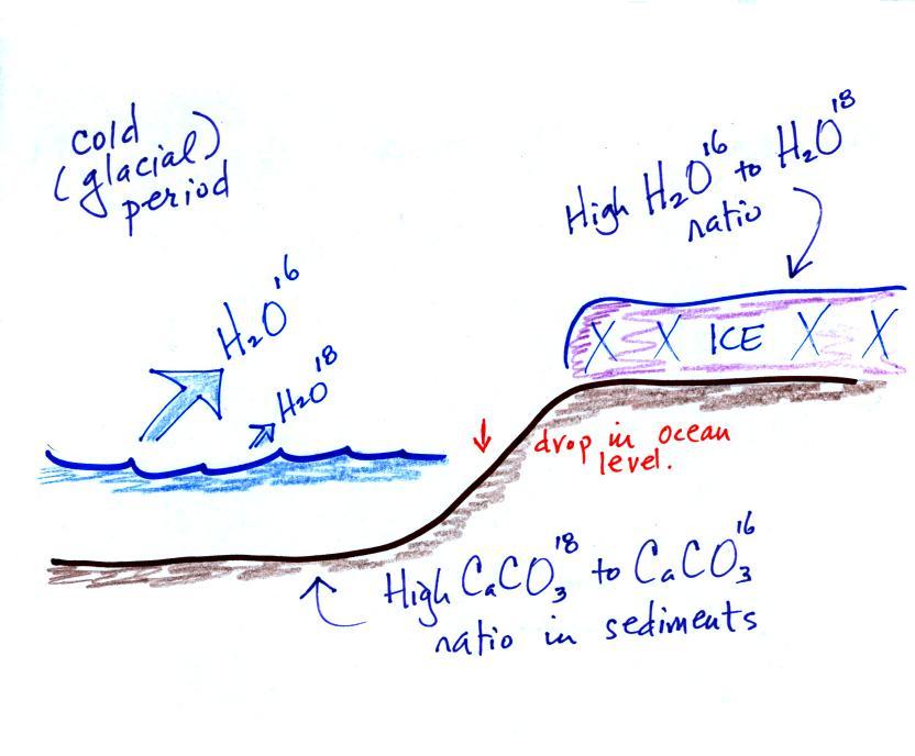
Core samples from ice sheets in Greenland and Antarctica were used to determine atmospheric carbon dioxide concentrations in the past. The ice can also be used to determine temperature. The basic idea is to determine the relative amounts of oxygen isotopes in the H2O that makes up ice.
Core samples from ice sheets in Greenland and Antarctica were used to determine atmospheric carbon dioxide concentrations in the past. The ice can also be used to determine temperature. The basic idea is to determine the relative amounts of oxygen isotopes in the H2O that makes up ice.
The
two
isotopes of oxygen contain
different numbers of neutrons in
their nuclei. Both
atoms have the same number of
protons.
During
a cold period, the somewhat
lighter H2O16
form of water evaporates more
rapidly than H2O18.
You would find relatively
large amounts of O16
in glacial ice. Since most
of the H2O18 remains
in the ocean, it is found in
relatively high amounts in calcium
carbonate in ocean
sediments. Note
also
the drop in ocean levels during
colder periods when much of the
ocean water is found in ice sheets
on land.
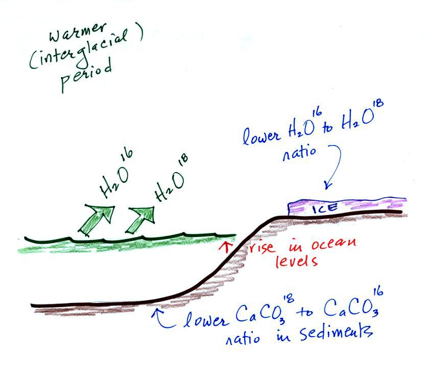
The
reverse is true during warmer
periods.
Coral can also be analyzed. Coral is made up of calcium carbonate, a molecule that contains oxygen. The relative amounts of the oxygen-16 and oxygen-18 isotopes depends on the temperature that existed at the time the coral grew.
4. 2000 year long temperature record
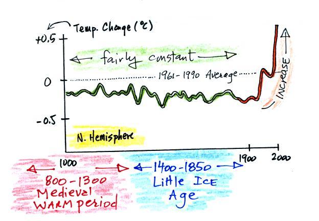
Using proxy data scientists have been able to estimate average surface temperatures for 100,000s of years into the past. The next figure shows what temperature has been doing since 1000 AD. This is for the northern hemisphere only, not the globe.
Coral can also be analyzed. Coral is made up of calcium carbonate, a molecule that contains oxygen. The relative amounts of the oxygen-16 and oxygen-18 isotopes depends on the temperature that existed at the time the coral grew.
4. 2000 year long temperature record
Using proxy data scientists have been able to estimate average surface temperatures for 100,000s of years into the past. The next figure shows what temperature has been doing since 1000 AD. This is for the northern hemisphere only, not the globe.
The
green
shaded portion of the
graph shows the estimates
of temperature (again
relative to the 1961-1990
mean) derived from proxy
data. The red shaded
portion shows the
instrumental measurements
were made between about
1850 and the present
day.
The figure above just shows the overall trend in temperatures during the past 1000 years. The actual data that the curve above is based on is shown below.
This is the so called "Hockey Stick Plot" originally published in 1999 by Mann, Bradley, and Hughes (and included in Climate Change 2001 - The Scientific Basis, Contribution of Working Group I to the 3rd Assessment Report of the Intergovernmental Panel on Climate Change (IPCC)).
Many scientists would argue that this graph is strong support of a connection between rising atmospheric greenhouse gas concentrations and recent global warming. Early in this time interval when CO2 concentration was constant, there are only modest changes in temperature. The largest overall change in temperature begins in about 1900 when we know an increase in atmospheric carbon dioxide concentrations was underway. The second half of the 20th century is the warmest period in at least the past 1000 years.
Some scientists have questioned the statistical methods used in the study. Additionally there is historical evidence in Europe of a medieval warm period lasting from 800 AD to - 1300 AD or so and a cold period, the "Little Ice Age, " which lasted from about 1400 AD to the mid 1800s. These are naturally caused changes in climate that are not clearly apparent in the temperature plot above. This leads some scientists to question the validity of this temperature reconstruction. Scientists also suggest that if large changes in climate such as the Medieval warm period and the Little Ice Age can occur naturally, then maybe the warming that is occurring at the present time also has a natural cause. There is also some question whether these were regional, not global, events.
The so-called Year Without a Summer is another example of a sudden short lived change in climate. It occurred in 1816, toward the end of the Little Ice Age. The unusually cold summer temperatures were apparently caused by a very large volcanic eruption the year before. Here's a short explanation of how volcanoes can cause short term cooling.
More recent temperature reconstructions have confirmed the overall trend shown in the figure above.
This is from the University of East Anglia Climatic Research Unit again.
The figure below shows results from 10 different research studies and extends the temperature reconstruction back 2000 years.
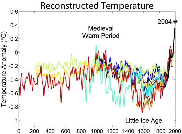
This figure was created for Global Warming Art by Robert A. Rohde and is discussed further here.
Somewhat larger temperature variations associated with the Medieval Warm Period and the Little Ice Age can be seen in this and the preceding figure. In both figures again the late 20th century has the warmest temperatures in the period.
We'll end this installment at this point. Here's a brief summary of where we stand:
There is general agreement that atmospheric CO2 and other greenhouse gas concentrations are increasing and that the earth is warming.
Not everyone agrees on the causes (natural or manmade) of the warming.
At times in the past the earth has been much warmer and also much colder than it is now. These changes all have natural causes. Before looking at how man might presently be causing climate to change we need to have a look at the climate history of the earth. That will be the topic of the next section in this series.
The figure above just shows the overall trend in temperatures during the past 1000 years. The actual data that the curve above is based on is shown below.
This is the so called "Hockey Stick Plot" originally published in 1999 by Mann, Bradley, and Hughes (and included in Climate Change 2001 - The Scientific Basis, Contribution of Working Group I to the 3rd Assessment Report of the Intergovernmental Panel on Climate Change (IPCC)).
Many scientists would argue that this graph is strong support of a connection between rising atmospheric greenhouse gas concentrations and recent global warming. Early in this time interval when CO2 concentration was constant, there are only modest changes in temperature. The largest overall change in temperature begins in about 1900 when we know an increase in atmospheric carbon dioxide concentrations was underway. The second half of the 20th century is the warmest period in at least the past 1000 years.
Some scientists have questioned the statistical methods used in the study. Additionally there is historical evidence in Europe of a medieval warm period lasting from 800 AD to - 1300 AD or so and a cold period, the "Little Ice Age, " which lasted from about 1400 AD to the mid 1800s. These are naturally caused changes in climate that are not clearly apparent in the temperature plot above. This leads some scientists to question the validity of this temperature reconstruction. Scientists also suggest that if large changes in climate such as the Medieval warm period and the Little Ice Age can occur naturally, then maybe the warming that is occurring at the present time also has a natural cause. There is also some question whether these were regional, not global, events.
The so-called Year Without a Summer is another example of a sudden short lived change in climate. It occurred in 1816, toward the end of the Little Ice Age. The unusually cold summer temperatures were apparently caused by a very large volcanic eruption the year before. Here's a short explanation of how volcanoes can cause short term cooling.
More recent temperature reconstructions have confirmed the overall trend shown in the figure above.
This is from the University of East Anglia Climatic Research Unit again.
The figure below shows results from 10 different research studies and extends the temperature reconstruction back 2000 years.
This figure was created for Global Warming Art by Robert A. Rohde and is discussed further here.
Somewhat larger temperature variations associated with the Medieval Warm Period and the Little Ice Age can be seen in this and the preceding figure. In both figures again the late 20th century has the warmest temperatures in the period.
We'll end this installment at this point. Here's a brief summary of where we stand:
There is general agreement that atmospheric CO2 and other greenhouse gas concentrations are increasing and that the earth is warming.
Not everyone agrees on the causes (natural or manmade) of the warming.
At times in the past the earth has been much warmer and also much colder than it is now. These changes all have natural causes. Before looking at how man might presently be causing climate to change we need to have a look at the climate history of the earth. That will be the topic of the next section in this series.