Information from Climate Models

Introdutory Notes on Climate Model Forecasts

Climate models are computer programs that are used to simulate Earth's climate and climate changes, including changes due to increased greenhouse gas concentrations. Climate models give us the only chance to properly account for the countless complex feedbacks and interactions that take place in the climate system and in particular how the system will respond to human greenhouse gas emissions. The information from climate models is an important consideration in the debate about the reasons for recent climate change as well as the projections for future climate changes in response to human emissions of greenhouse gases. The model results can be considered the best estimates based on the work of the community of expert scientists who have developed and improved the models.

Yet, keep in mind that these models are not reality. There is much that we do not understand about the operation of the climate system on Earth, for example, some of the complex feedbacks mentioned on the previous page. We certainly cannot program models to be more accurate than our understanding of the underlying processes. There are also many important processes that happen over space and time scales that are not resolved by these models, such as cloud formation. The impact of these unresolved processes must be parameterized. Model results can be highly dependent on these parameterizations. Parameters need to be "tuned" to achieve desired results. For example, models can be tuned to try to match past, known temperature changes.

Thus, the models are not perfect and do not make exact predictions. Simulations made by these models are one tool we have to help understand climate and climate change on Earth. Given that climate model predictions are uncertain, we should also consider other sources of information when deciding environmental policy. In other words, the results of climate model simulations should not be the sole reason for enacting environmental policy.

Climate models are used to help answer the question of "attribution" as well as make predictions about Earth's future climate. Attribution studies examine the question of whether recently observed climate changes can be attributed to natural variations or to greenhouse gas emissions. In this class we will focus on attribution with respect to the observed changed in global average surface temperature over the past 100 years or so. There are also attribution studies being done with respect to individual severe weather events, such as the heat wave in western North America in 2021 and several Atlantic Hurricanes over the past couple of years. We will not cover this aspect of attribution in much detail.

Models are also used to make predictions about how climate will change in the future based on several different senarios for future human greenhouse gas emissions.

Attribution of Recent Warming based on Climate Models

The information on climate model results presented in this section comes from the report, Climate Change 2013: The Physical Science Basis, which is part of the Fifth Assessment Report of the Intergovernmental Panel on Climate Change (IPCC). The discussion of attribution is contained in chapter 10 of the report, "Detection and Attribution of Climate Change: from Global to Regional." The Sixth Assessment Reports have been being released during the last year and have not been incorporated into this section. However, little has changed with the information and conclusions in relating greenhouse gas emissions and climate change.

Before presenting graphical information about attribution, here are several statements taken from the executive summary in chapter 10:

It is extremely likely that human activities caused more than half of the observed increase in Global Mean Surface Temperature (GMST) from 1951 to 2010.

GHGs contributed a global mean surface warming likely to be between 0.5°C and 1.3°C over the period 1951–2010, with the contributions from other anthropogenic forcings likely to be between −0.6°C and 0.1°C, from natural forcings likely to be between −0.1°C and 0.1°C, and from internal variability likely to be between −0.1°C and 0.1°C.

Robustness of detection and attribution of global-scale warming is subject to models correctly simulating internal variability.

The IPCC report defines "extremely likely" as (95–100)% confidence and "likely" as (66–100)% confidence. The climate models used in the IPCC assessment strongly suggest that much of the observed increase in GMST since 1951 is due to increases in GHGs in the atmosphere and not due to natural climate change. The models indicate that GHG increases caused a warming of between 0.5°C and 1.3°C over the period 1951–2010, while natural forcings and internal variability have had a much smaller impact in the range of −0.1°C and 0.1°C. The third quote above states that climate models' assessements of attribution rely on the models' abilities to correctly account for natural variability or how climate changes without any changes in greenhouse gases. Critics of climate models claim that they do not properly simulate natural changes in climate.

The IPCC assessment includes 20 climate modeling groups that run over 60 different models as part of the Coupled Model Intercomparison Project (CMIP). One goal of these studies is to evaluate how realistically the models simulate past climate. Global average surface temperature can be estimated from direct measurements from about 1860 to present. Prior to that there were not enough direct measurements. The CMIP climate models are configured to simulate Earth's climate from 1860 to present to test how accurately they can simulate the known changes in temperature after 1860. These simulations can include natural factors or forcings, such as volcanic erruptions and changes in solar radiation. Greenhouse gas concentrations in the model are set to match the known increases in greenhouse gases as the model runs forward in time after 1860. A nice feature of using computer models is that the models can be run again, but without changing the concentration of GHGs in the atmosphere after 1860, i.e., without including human emissions of GHGs. This provides the possibility of separating the impacts of GHGs emissions from natural climate change as shown in the figures below.

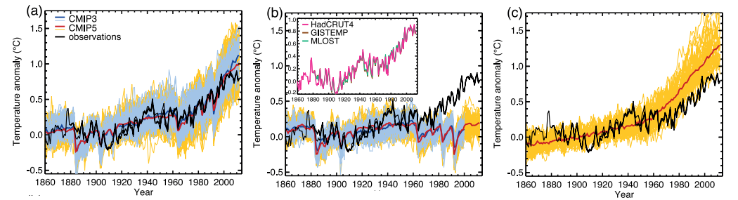Figure 10.1, panels a, b, and c taken from Climate Change 2013: The Physical Science Basis. In all panels, the horizontal axis is the model year and the vertical axis represents the change in global average surface temperature relative to the average temperature over the period from 1880–1919. Thin blue lines show individual model results for the CMIP3 experiment and thin yellow lines show individual model results for the CMIP5 experiment. Thick light blue and red lines show the average of all the CMIP3 and CMIP5 model runs. The thick black line shows the observed temperature change, which is based on the average of three different estimates. In panel (a), all human and natural forcings are included in the model runs. Panel (b) includes only natural forcings with no change in GHGs or other human forcings. Panel (c) includes only GHG forcings with natural forcings removed and no other human forcings considered. Refer to original source for more detail.

The figures are taken directly from the latest IPCC report as indicated in the caption. Figure 10.1 (a) shows that climate models have generally been able to reproduce the observed changes in temperature over the period from 1860–2010. This is a significant test of the models' abilities to simulate past changes in global average temperature. Figure 10.1 (b) shows the models' simulations of the change in temperature when natural forcings are included, but GHGs are held constant at 1860 levels. Notice that the observed temperature change (thick black line) is significantly larger than the temperature change simulated by the models when the models do not include GHG increases (particularly after 1980). According to these climate models, natural changes in global average surface temperature would have been less than 0.1°C without human greenhouse gas emissions and other human forcings. Panel (c) shows the models' simulations with greenhouse gas increases included, but without natural forcings or other human forcings. For this case, the models simulate more warming than has been observed after 1980. This is because the models simulate an overall cooling impact from other human forcings, such as land use changes and aerosol emissions. In other words, without other human climate forcings that have acted to cool the GMST, the global average temperature would about 0.5°C warmer than it is today (according to climate model predictions). With regard to attitribution, climate models strongly support that most of the observed increase in global average surface temperature since 1860 is due to increases in GHGs and the increase in temperature would not have happened without human emissions of greenhouse gases.

One thing to point out is that predictions of future climate change are much more difficult than simulating past climate changes where the answers are basically known beforehand. This allows modelers to tweak their models until they get the "known" answer. In this case the change in global average temperature that took place from 1860 to 2010 was known, and models could be tested and developed to get this answer. There is a question of whether or not the models got the "known" answer for the right reasons. Some argue that much of the warming over the last 100 years was due to natural reasons not related to greenhouse gas emissions and that the models do not properly simulate natural climate cycles. Therefore, in order for the models to reproduce the observed warming from 1860 to 2010, they were programmed to be overly sensitive to human emissions of greenhouse gases. The more sensitive the models to increases in greenhouse gases, the more warming that is predicted due to future emissions of greenhouse gases. Of course when making predictions of future climate changes, one does not know the answer beforehand. But if current models are tuned to be overly sensitive to greenhouse gas emissions, then future predictions of increases in surface temperature due to greenhouse gas emissions will be too large.

In addition, the model's representation of Earth's climate is not reality. There no point during a simulation where the model's representation of the climate matches a known measured state of the climate. If you do try to initialize the model to some point in history, it will revert back to the model's perception of climate. Thus, while climate modelers were able to reproduce the overall change in global average temperature after adding greenhouse gases within the model world, it requires a big leap of faith to believe the same overall change would happen in the real climate system simply due to the addition of greenhouse gases. One problem with climate model simlations is that they generally fail to reproduce the temporal (time) and spatial (position) variability that is known to happen in the real world, especially over small scales. This "natural variablity" is observed in nature but not so much in climate models. In other words, the models seem to underestimate natural changes in climate that happen without changes in greenhouse gases, and may overestimate changes in climate that result from changes in greenhouse gases. It is quite possible that the observed increase in temperature over the last 100 years has been wrongly attributed to the increase in greenhouse gases by climate models. Perhaps the observed change in global average temperature was part of a natural climate change and not dominated by the increase in greenhouse gases.

In order to make this point, a few lines written by Dr. Kevin Trenberth a senior climate change researcher working for the National Center for Atmospheric Research, which was orginally posted on a blog from Nature Climate Change will be discussed. The following statements were quoted from the blog, "In particular, the state of the oceans, sea ice, and soil moisture has no relationship to the observed state at any recent time in any of the IPCC models" and "None of the models used by IPCC are initialized to the observed state and none of the climate states in the models correspond even remotely to the current observed climate" both indicate that a climate model is not the real world. Therefore, starting a model in the year 1900 does not mean that the climate model looks anything like the year 1900. It just means starting the model with year 1900 greenhouse gas concentrations. It is misleading to believe that climate models have been able to reproduce the climate that happened from 1900 to 2000. The claim is that the change in global average temperature simulated by the models in response to adding greenhouse gases is the same as the change in global average temperature in the real world. Quoting from the blog, "The current projection method works to the extent it does because it utilizes differences from one time to another and the main model bias and systematic errors are thereby subtracted out. This assumes linearity." There are plenty of scientists who disagree with this last statement that the "errors" will necessarily subtract out. There are certainly important processes within the operation of the climate system that are themselves highly non-linear. Finally, considering the uncertainty in current model predictions, Trenberth said, "We will adapt to climate change. The question is whether it will be planned or not?" This indicates to me that unless we are able to improve the predicitons of current models, we are just going to have to adapt to climate changes without knowing what is coming. Instructor's Note: I include the quotes from Dr. Trenberth, who is an expert in climate modeling, because I have been criticized in the past for making similar comments about climate models. The quotes were not meant as an attack on Dr. Trenberth, who is a highly competent scientist. These were included to make a point that is not often made clear to the public.

Climate models continue to evolve and improve due to increases in computing power and improved observations and understanding of the climate system. However, the predictions of current climate models should be viewed with scientific skepticism. We do not have time to discuss this topic in much detail. If you are interested in the basics of climate model simulations including reasons why the models produce uncertain predictions, you may want to read, Climate Models for the Layman by Dr. Judieth Curry. ATMO 3336 students are not required to read the document.

Predictions of Equilibrium Temperature after doubling CO₂

There are many different climate models and different models make different predictions about the future. The reason is that no model can fully represent all the complex process and feedbacks involved in the Earth system. Due to this uncertainty, we should consider all of them as possible outcomes of adding greenhouse gases. There is also a realistic possibility that all models will turn out to be wrong. Perhaps the climate changes due to adding greenhouse gases will be less severe than predicted by models or perhaps we will be surprised and climate changes will be more severe than predicted by current models.

The ability of global climate models to reproduce the observed surface temperature trends over the 20th century represents an important test of the models. While most climate models are able to reproduce the warming in global average surface temperature that has been measured since 1860, no model is able to correctly get the spatial patterns of temperature changes correct. In other words, the observed changes in climates at the scale of regional climate zones has not been reproduced by any climate model.

The Intergovernmental Panel on Climate Change (IPCC) has released a set of reports, which comprises the Fifth Assessment Report (AR5) on climate change. Material from the Summary for Policymakers will be referenced in this section. As reported in the 2013 IPCC Report, various modeling studies have suggested that a doubling of atmospheric carbon dioxide from it pre-industrial value of 280 ppm to 560 ppm, or its equivalent by incorporating the effects of increases in other greenhouse gases, will likely increase mean global temperatures between 1.5 and 4.5°C, with a mean value of 3°C. It is also extremely unlikely that the increase in temperature will be less than 1°C and very unlikely greater than 6°C. According to the report, likely means probability >66%, extremely unlikely means <5%, and very unlikely means <10%. Recall that the non-feedback calculation for the increase in global average temperature after carbon dioxide has doubled from 280 ppm to 560 ppm is 1°C. This means that most of the climate models used to produce the 2013 IPCC Report have fairly strong positive feedbacks with respect to changes in carbon dioxide (greenhouse gases), since the most likely outcome (from climate models) is that if CO₂ were doubled, the global average temperature would increase by 3°C, which is much more than 1°C that has been estimated for the "non feedback" case.

Recall from the previous page that most current climate models have a strong positive feedback with respect to temperature changes initiated by increasing greenhouse gases. Specifically, much of the predicted warming in climate model simulations is not directly caused by human emissions of greenhouse gases, but happens as a result of positive feedbacks in the models that are related to changes in water vapor and clouds. As pointed out on the previous page, models are known to have problems in accutately representing the movement of water vapor and the formation of clouds. Thus, two process that are not well represented in climate models, i.e., have a lot of uncertainty, end up being responsible for much of the predicted overall warming. The point is that current climate model predictions concerning the magnitude of the overall warming that may result from human emissions of greenhouse gases are far from fact and should be considered uncertain predictions. This is not to say that the net internal feedbacks might not be positive. They may very well be. But there are many who believe that models overestimate the net positive feedback. In other words, the model simulations end up being too sensitive to increases in greenhouse gases and may predict more warming than will take place in the real world.

You should understand that these studies are done by instantly doubling carbon dioxide in the model, then letting the model run until a new equilibrium climate state is reached. In reality, the increases in greenhouse gases happen over an extended period of time and the climate system takes some time to come into equilibrium. A big issue here is that the warming in surface temperatures tends to lag behind the increase in greenhouse gases. To a large degree, this lag is due to the large thermal inertia of the oceans -- in other words it takes a lot of energy to raise the temperature of the ocean water.

Let's try to break it down into understandable steps.

• Increasing the amount of greenhouse gases in the atmosphere, intially slows down the rate at which the Earth emits infrared radiation to space.
• Assuming no change in energy input (Energy the Earth absorbs from the Sun), the Earth is no longer in energy balance since energy in exceeds energy out.
• As long as energy in exceeds energy out, the planet warms. In particular the Earth's surface temperature will warm.
• As the Earth's surface temperature warms, the amount of radiation energy it emits increases. Since some of this extra radiation energy is lost to space, thus the amount of radiation energy that the planet emits to space starts to increase.
• The warming continues until the energy out increases to the point where it equals the energy input.
• The Earth's surface is 70% covered by Oceans. Oceans have a high thermal inertia, so the Ocean surface temperature is slow to warm up in response to the energy imbalance caused by adding greenhouse gases to the atmosphere. The two main reasons for this is that (1) water has a high specific heat (meaning you have to add a lot of energy to liquid water to change its temperature in comparison to many other materials), and (2) the surface temperature of the ocean is slow to warm up because the additional heat is able to mix somewhat through the entire depth of the oceans.
• Therefore the amount of warming of the Earth's surface (temperature increase) required to bring the system back into balance (energy input equal energy output) will take quite some time.

Some estimate that the atmospheric concentration of CO₂ will reach 560 ppm (double the pre-industrial level) by the year 2060. However, as a result of the delay induced by the oceans, climate models do not predict that the Earth to warm by the full 1.5-4.5°C (2.7-8.1°F) by 2060. Assuming this delay is real, we can make several conclusions here.

1. This delay provides an opportunity to reduce the magnitude of anthropogenic climate change before it is fully realized, if appropriate action could somehow be taken to reduce greenhouse gas concentrations. This would require us to take CO₂ out of the atmosphere.
2. Even if we were to stabalize greenhouse gas concentrations today by completely eliminating new emissions, this delay means that the surface temperature will continue to warm until a new equilibrium is reached (this may take a hundred years or more).
3. If we wait to act, still greater climate change will be expected, which will be more difficult or impossible to avoid.
4. The ocean surface temperature would also be slow to cool. Suppose in the future climate change gets out of control and we decide that we need to lower the average surface temperature of the Earth by somehow removing greenhouse gases from the atmosphere. The cooling would be very slow and lag behind the decrease in greenhouse gases. Thus anthropogenic global warming, if it takes place, cannot be quickly reversed.

Climate Sensitivity: A Quick Look at the Latest Generation of Models

This section was just added based on an interesting study on the CMIP 6 models. I tried to make it understandable for all students. Please do not worry if you find it difficult. You will not be specifically tested on this material. I hope you find it interesting.

The IPCC has released its Sixth Assessment Report (AR6) within the last year. The Fifth Assessment Report (AR5) was published in 2013. Part of each assessment includes a Coupled Model Intercomparison Project (CMIP) to gather and compare predictions from different climate modeling groups. In the 5^th Assessment Report, the CMIP5 models predicted that the Equilibrium Climate Response for a doubling of CO₂ would be a warming of Global Average Surface Temperature (GAST) in a range from (2.0 - 4.7)° C. {The range specified in the previous section (1.5 - 4.5)° C was from the IPCC AR4 report in 2007}. A new paper, Compensation Between Cloud Feedback and Aerosol-Cloud Interaction in CMIP6 Models published Jan. 25, 2021 in the journal Geophysical Research Letters by Wang et al. has come out with some preliminary results from the ongoing CMIP6 studies.

Interestingly, the spread of the model predictions for the equilibrium warming of GAST for doubled CO₂ has increased to (1.8 - 5.5)°C with a mean of 3.7°C. [It hardly seems like the "science is settled" on this issue as many claim. It looks like the uncertainty regarding the climate response to increasing GHGs has grown (at least according to the latest generation of climate models)].

CMIP6 models that predict the most warming are those that are most sensitive to increases in GHGs, while less sensitive models predict less warming. Interestingly, all models are able to generally reproduce the known changes in GAST over the 20^th when including the known increases in GHG concentrations. In part this is possible because models also simulate cooling from human-produced aerosols. Without going into details, human-produced aerosols are simulated to have a cooling impact on climate mainly because they can act as cloud condensation nuclei (CCN). The "extra" CCN aerosols cause low altitude clouds to form with more smaller droplets rather than fewer large droplets. This results in (a) clouds being more reflective of visible radiation from the sun and (b) clouds persisting longer before raining or evaporating. Both of these effects have a cooling influence on GAST.

Models with high warming sensitivity to increasing GHGs generally also have higher cooling sensitivity to aerosols, while models with low sensitivity to GHGs also have low sensitivity to aerosols. This balancing act allows both high and low sensitivity models to reproduce the known changes in GAST in the 20^th century by tuning the models to match the specified temperature changes. The parameterization of aerosol impacts on cloud properties provides one set of tunable parameters in the models.

Not only are simulations of cloud-aerosol properties highly uncertain, but the amount of human-produced aerosol released and the evolution of the aerosols in the atmosphere are uncertain. A question that we will consider later is the reason for the observed decrease in GAST from about 1940 - 1980 during a time when GHGs were increasing. Some climate models attribute this to the cooling influence of human-produced sulfate aerosols from coal burning. As coal buring was reduced and cleaned up in much of the western world after 1980, models simulate less aerosol released and less cooling impact, which results in the rapid warming after 1980. The models with the highest sensitivity to GHG increases predict the largest future increases in GAST in combination with expected decreases in human aerosol pollution.

Wang et al. (2021) looked more closely at how well high and low sensitivity models were able to reproduce the observed changes in temperature over the 20^th century. While both were able to somewhat reproduce the observed changes in GAST (differences between the models are mostly insignificant wrt GAST), there are statistically significant differences between the Northern Hemisphere and Southern Hemisphere temperature changes simulated by the models. This is because the majority of human-produced aerosols are released in the Northern Hemisphere. Unlike CO₂, which spreads around the entire globe, aerosols are mostly washed out of the atmosphere before they are able to spread from the Northern to Southern Hemisphere. Thus, the cooling impact of aerosols is strongest in the Nothern Hemisphere. Compared to the measured change in temperature in the middle to late 20^th century, the high sensitivity models simulate too much warming in the Southern Hemisphere and too little warming in the Northern Hemisphere. The low sensitivity models agree much better with the observed temperature changes in both the Northern and Southern Hemispheres. Only 5 of the 30 CMIP6 models analyzed are classified as low sensitivity. For those 5 models, the equilibrium temperature change for a doubling of CO₂ ranges from (1.8 - 2.9)°C, with a mean of 2.5°C. This is far lower than the 3.7°C mean for all 30 models. The most sensitive CMIP6 model estimates that the equilibrium temperature would increase by 5.5°C for a doubling of CO₂. There continues to be a wide range of estimate (that may even be growing) from climate models concerning how the Earth's surface temperature will change in response to increasing GHGs. Based on results of this study, climate models with lower sensitivity to increasing GHGs and thus lower estimates of equilibrium warming for doubled CO₂ were shown to more accuratley reproduce the observed hemispherical pattern of temperature changes over the 20^th century.

Model Predictions of Global Average Temperature Changes for the 21^st Century

In the 2013 IPCC Summary for Policymakers it is stated that the global average temperature change for the period 2016 - 2035 relative to the 1986 - 2005 period will likely be in the range 0.3°C to 0.7°C warmer. The models predict an average rate of warming of 0.17°C per decade over this period. The 2007 IPCC report stated that even if concentratrations of all greenhouse gases had been kept constant at year 2000 levels, a further warming of at least 0.1°C would still be expected by the years 2016 - 2035 [due to the ocean delay]. Therefore, the near term prediction is for warming even if we reduce (or eliminate) emissions of greenhouse gases. The 2013 IPCC document addresses the issue of climate change commitment and irreversibility. If climate model predictions are correct, then each year that CO₂ increases means a commitment to some higher level of temperature in the future, which cannot be easily reduced or reversed without some way to remove large quantities of CO₂ from the atmosphere. Quoting from section E.8 of the 2013 IPCC Summary for Policymakers:

Cumulative emissions of CO₂ largely determine global mean surface warming by the late 21st century and beyond. Most aspects of climate change [that result from human emissions of greenhouse gases] will persist for many centuries even if emissions of CO₂ are stopped. This represents a substantial multi-century climate change commitment created by past, present, and future emissions of CO₂.

A big problem in making predictions of longer term future climate change is uncertainty regarding future greenhouse gas emissions. The uncertainty encompasses substantial unknowns in population and economic growth, technological developments and transfer, and political and social changes. The IPCC addresses this issue by running models over a wide range of future emission senarios called Representative Concentration Pathways (RCPs) as shown in the figure below. RCP8.5 represents a future with little reduction of emissions, with a CO2 concentration continuing to rapidly rise, reaching 940 ppm by 2100. RCP6.0 has lower emissions, achieved by application of some mitigation strategies and technologies. CO₂ concentration rising less rapidly (than RCP8.5), but still reaching 660 ppm by 2100. In RCP4.5, CO₂ concentrations are slightly above those of RCP6.0 until after mid-century, but emissions peak earlier (around 2040), and the CO₂ concentration reaches 540 ppm by 2100. RCP2.6 is the most ambitious mitigation scenario, with emissions peaking early in the century (around 2020), then rapidly declining. Such a pathway would require early participation from all emitters, including developing countries, as well as the application of technologies for actively removing carbon dioxide from the atmosphere. The CO₂ concentration reaches 440 ppm by 2040 then slowly declines to 420 ppm by 2100.

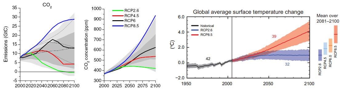Left plot shows projected emissions of CO2 based on the four different emission senarios tested by the IPCC through 2100. Middle plot shows expected atmospheric concentration of CO2 for the four RCPs. Right plot shows the simulations of the CMIP5 models from 1950 to 2100 for each of the RCPs. Historical CO2 concentrations are used from 1950 to 2005 and RCPs after 2005. The vertical axis is the change in global average surface temperature relative to the average temperature for 1986–2005. Prediction of future climate changes depend heavily on the emission senario selected, especially after 2030 when the emission senarios diverge greatly. Only RCP2.6 and RCP8.5 are plotted. Heavy line is the CMIP model average and shading shows the range of model predictions. The mean and associated uncertainties averaged over 2081-2100 are given for all RCP scenarios as colored vertical bars.

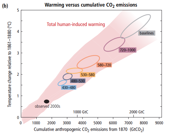
Based on the figure above, the Intergovernmental Panel on Climate Change (IPCC) projects a warming of 0.3-4.8°C (0.5-8.6°F) in global average temperature for the last two decades of this century (2081 - 2100) relative to the average temperature for 1985 - 2005. This estimate is based on the latest runs of what are considered to be the best global climate models and a wide range of estimates of future emissions of greenhouse gases. Some have been critical of this large range of predictions from models, complaining that the uncertainty is too large to help with policy decisions. However, the biggest reason for the large range in the predicted temperature change is the large uncertainty in future emissions. The model predictions have much less spread for known increases in greenhouse gases. In fact, the model predictions for changes in temperature are most influenced by the cumulative (total) greenhouse gas emissions since 1860, which is something that we humans have under our control. The figure below is figure SPM.5(b) taken from the IPCC report, Climate Change 2014 Synthesis Report Summary for Policymakers. The horizonal axis is the cumulative emissions of CO₂ since 1870 in units of Gigatons (billions of tons). The vertical axis is the simulated temperature change relative to the average temperature for 1861–1880. The pink shaded region shows a nearly linear relationship between the amount of warming predicted by the CMIP5 models and the total emissions of CO₂. The black oval indicates the cumulative emissions by the year 2005 (about 1800 Gigatons) and the corresponding observed temperature increase of about 0.8°C above the 1861 to 1880 average. This oval falls well within the pink range of predictions from the models. The remaining ovals show the most probable corresponding ranges of total future CO₂ emissions and temperature changes based on the CMIP5 models. This figure shows that climate model predictions of future temperature change are sensitive to the historical total amount of GHG emissions ... and the temperature will continue to rise nearly linearly with the accumulated emissions.

Evaluation of Climate Model Predictions after 2005

The first IPCC report in 1990 projected a warming of global average temperature of between 0.15 and 0.30°C per decade from 1990 to 2005. This can now be compared to the observed value of 0.20°C per decade as determined from satellite measurements (see figures below). The success of this early prediction through the end of the 1990s led many to have confidence in the ability of climate models to predict changes in global average temperture due to increasing greenhouse gases. However, the relatively rapid warming trend that took place in the late 1990s seemed to slow down in the early 2000s, and this was not predicted by most of the IPCC climate models.

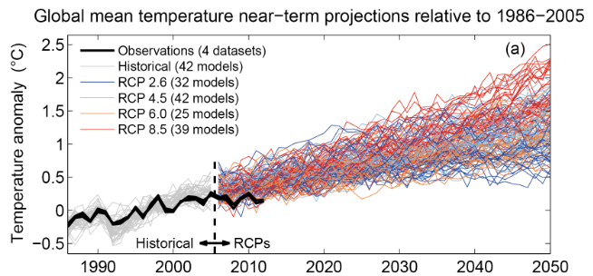
The set of figures below are based on the 2013 IPCC report. In this case from the AR5 simulations, the climate model runs were forced with the known (measured) increases in greenhouse gases up until the year 2005. After 2005, the models make predictions based on various estimates for how greenhouse gases would increase. The temperature anomaly graphed in these plots is the change in global average surface temperature relative to the global avearage temperature from 1986 to 2005. The portion of the model runs prior to 2005 is known as a "hindcast" since the modelers knew both the actual increase in temperature (from observations) and used the actual increases in greenhouse gases (measured). The individual model runs are shown with thin grey lines. (Note: models were "tuned" to produce a temperature change that was very close to the observed temperature change. This part is not a true forecast.) After 2005, the models used various estimates for how greenhouse gases would increase. The actual temperature change is not known by the modelers, so temperature changes after 2005 are predictions. Individual predictions from the different model runs are shown using thin colored lines. The bold black lines in the figures show the observed change in global average surface temperature based on 4 different observational datasets.

The figure on the left is taken directly from the IPCC report. The report was published in 2013. Thus, the observational data only runs through 2012. The observed change in temperature is near the lower portion of all the model predictions. Some claim this plot is misleading because 2012 was near the end of the "pause in global warming." The figure on the right updates the observational data through May 2022. The observations now contain the warmer years after 2014. Around 2016, the observed change in global average temperature was nearer to the middle range of the model projections. However, the global average temperature has not risen after 2016 and at the time of the latest update (May 2022), the observed global average surface temperature is near the bottom of the range of predictions made by models in 2005. We are currently in an extended La Nina pattern (discussed below), which likely contributes to keeping the global average temperature down. Some predict that we are due for a strong El Nino pattern, which could result in another period of rapid warming.

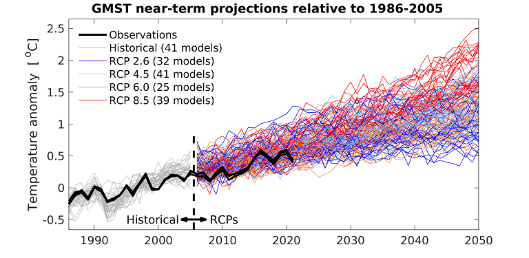The image on the left is figure 11-25A from the IPCC's Fifth Assessment Report, which shows changes in global average temperature relative to the 1986 to 2005 average (labeled as temperature anomaly). The bold black lines show the the temperature anomaly as determined from four different measured datasets of global average surface temperature. The individual thin lines show the output from climate models run by the IPCC. The model simulations were run in 2005. Model output from 1986 to 2005 (grey lines) are known as "hindcasts" since the simulation covers years that have already passed. Hindcasts are often used to test whether a model was able to closely simulate past times when the temperature changes are known. Since the past temperature changes are known, modelers are able to "tune" their models to match these past changes. The individual model lines are colored after 2005 to indicate that these are true forecasts of future temperature change. The last year for the observational data in this figure is 2012. The figure on the right has been updated to include observational data through May 2022. (Source: the Climate Lab Book)

A Look at the Satellite-Derived Temperature Record

During and just after the "pause in global warming" from 2002 to 2013, some wondered if the global average temperature would continue to be steady or even turn around and begin a period of cooling. Based on observations, we can now say that the global average temperature definitely increased after the pause. The figure below shows the satellite-derived changes in the monthly global average temperature from January 1979 through February 2023. The approximate period of the "pause in global warming" is marked in green. The red line shows a smoothed version of the month to month temperature changes by averaging over 13 months. The current end point of the red line shows that the 13 month smoothed global average temperature is about 0.1 to 0.2°C warmer than the global average temperature during the pause period. The last point on the red line corresponds to September 2022. Note that the satellite-derived temperature has been oscillating up and down over the last 7 years (since 2015), though the average temperature is a few tenths of a degree warmer than the average during the pause period. The linear trend for the entire satellite record (from January 1979 to March 2022) is +0.13°C per decade. However, the observed temperature changes are far from linear. There are obviously shorter periods of increasing and decreasing temperature superimposed on the longer term linear increase. Thus, caution should always be exercised when extrapolating short term temperature trends into the future. While the latest temperature is near the bottom of the recent oscillations, we can expect this to turn around to warming once the current La Nina cycle ends as discussed below.

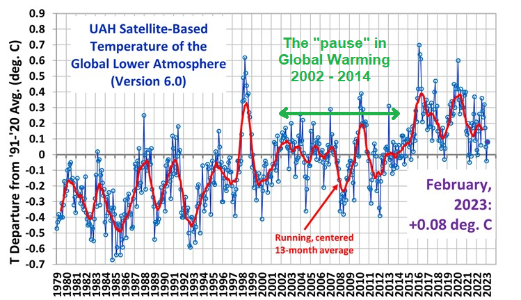Monthly changes in the global average temperature of the lower atmosphere based on satellite observations from 1979 to February 2023 relative to the average temperature from 1991 to 2020. Blue circles show the temperature differece each month. The red line is smoothed using a 13 month centered average. The approximate period of the "pause in global warming" in green was added by Dr. Ward. ( Source for the original figure)

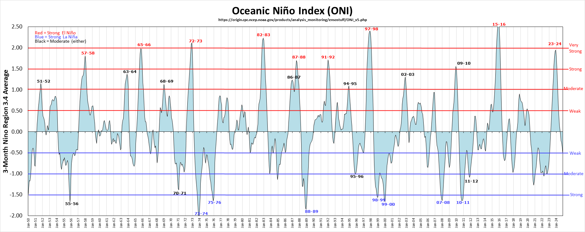
The short-term variations in warming and cooling are influenced by natural climate fluctuations associated with the El Nino / La Nina climate cycles. Without going into details, it is common for global average temperature to spike upward during El Nino years and then come back down the La Nina portion of the cycle. The Oceanic Nino Index from 1950 through present shows the past pattern of this cycle. (A little more detail on the El Nino cycle is provided in a later reading page). There was a strong El Nino in 1997/1998 followed by a strong La Nina in 1999/2000, which corresponds with a strong warming period followed by a strong cooling period in the satellite-derived global average temperature. More recently, there was a strong El Nino in 2015/2016 followed by a La Nina in 2017/2018, then a weaker El Nino in 2018/2019 followed by the current moderate La Nina that began in late 2020. The figure above shows a relatively sharp drop in the satellite-derived global average temperature in the last couple of years due to the current La Nina, which has persisted for nearly 3 years.

Quick Update for Fall 2023

Normally, I update past temperature information in the spring semester after the year end data becomes available. However, as you may have heard, a significant increase in GAST has been observed since the start of the summer. At least part of that is due to the shift from La Nina to El Nino conditions in the Pacific. The satellite-derived temperature record discussed above has jumped to its highest positive monthly anomaly every observed (since this data became available January 1979). The most recent month, September 2023, is clearly higher than the previous peaks associated with the strong El Ninos in 2016 and 1998, and may continue to climb if the El Nino strengthens. Link to plot through September 2023 . Note that the satellite-derived temperature record is not the same as the "official" records of GAST from ground observations. Updates of the officical records take more time to process and will not be available until next year. But it seems like a good chance that 2023 will have the highest GAST since records began around 1860.

Concluding Thoughts on Climate Model Simulations of Recent Changes in GAST

As we will discuss soon, the Earth's climate has changed naturally throughout its history with both warming and cooling periods. There were times in the past when it was much colder than today and times in the past when it was much warmer than today. Changes in greenhouse gas concentrations are just one of many factors that influence the global average temperature. The changes we are observing now are due to a combination of natural climate change and human-caused increases in greenhouse gases. We cannot separate these effects, i.e., we do not know how the climate would have changed if greenhouse gases did not increase. We expect that increasing greenhouse gases will be a warming influence. But is all (or even most) of the recent warming due to greenhouse gas increases? Or is most of the recent warming simply part of a natural cycle of warming without much influence from greenhouse gas increases? The answer to these questions remains uncertain. According to climate models, the recent warming is almost entirely due to greenhouse gas increases because if the same models are run without increasing greenhouse gases, they do not simulate increasing temperature. But if the recent warming is natural and the models incorrectly attribute warming to greenhouse gases, then they will likely overpredict future warming as greenhouse gases continue to increase, i.e., the simulations may be overly sensitive to increases in greenhouse gases. The amount of future warming is very important in deciding future policies regarding greenhouse gas emissions. If the warming from greenhouse gases is small, then perhaps the benefits of using fossil fuels outweighs the harms or risks. However, if the warming from greenhouse gases is large, then the prudent course of action would be to severely reduce future emissions. Based on the presentation above, it seems that most models have been predicting more warming than has been measured. The reason for this discrepancy is not fully understood. The Earth's climate system is very complex and difficult (some say impossible) to accurately model. Will models continue to overpredict future warming? The answer to that question is important but uncertain.

Climate Model Predictions for Climate Changes at Regional Scales

In previous semesters, I would point out that while all climate models predict warming of the global average temperature (giving us relatively high confidence that human emissions of greenhouse gases will result in global warming, although the magnitude of the warming remains uncertain), individual model predictions are all over the place when you look at regional scale (small spatial scale) predictions for changes in temperature and precipitation (giving us low confidence in the ability of climate models to project regional climate changes). In other words, two models that predict similar changes in global average temperature will often have vastly different predictions for climate changes that might happen over smaller regions, such as the Senoran Desert region for example. In spite of the difficulty in being able to predict climate changes that may occur over regional scales, accurate predictions of climate changes over regional scales are very important in understanding and preparing for how climate change will ultimately impact humans and other life. Life will be more impacted by changes on regional scales where the life exists, rather than changes in global average temperature.

The latest IPCC Report claims that there is now higher confidence in projected patterns of warming and other regional-scale features, including changes in wind patterns, precipitation, and some aspects of extremes. I do not have time to evaluate the IPCC claim that regional projections from climate models are becoming more accurate and trustworthy. Here is a paraphrased summary taken from the most recent IPCC report: In summary, IPCC Fifth Assessment projects that warming in the 21st century will continue to show geographical patterns of warming similar to those observed over the past several decades, i.e., warming is expected to be greater over land than ocean, and the high northern hemisphere latitudes (Arctic) will warm more rapidly than the global average. In spite of recent improvements in the regional scale predictions, climate models continue to have major problems in reproducing the multi-decadal climate variability that is known (through observations) to take place at regional (ecosystem-level) scales. Since global scale changes can be considered as a summation and interaction of regional climate changes, many question whether current climate models are even capable of accurately predicting future climate changes until they can better simulate natural variability and regional-scale climates.

Instructor's note. Simulation of regional climate changes continues to be an area of active debate. I attended a seminar recently in which the speaker argued that regional scale climate changes have a significant random component to them, i.e., over short time scales (decades), random and unpredictable changes in circulation patterns have a large influence on regional climate changes. If this is true, there may be a fundamental limit to how well regional scale climate changes can be predicted over a specific decadal time period, and perhaps some are expecting more from climate models with repsect to regional climate change than they can possibly deliver. However, one may be able to separate the random components of regional climate change from the global climate change forced by adding greenhouse gases. This again raises the possibility that climate models may be able to somewhat accurately predict the increase in global average temperature due to increasing greenhouse gases, but have little skill in predicting changes over smaller regional areas. In fact, the speaker was running "ensembles" of climate models, similar to ensemble weather forecasting that we covered earlier in the semester, which indicated a whole range of equally possible outcomes at regional spatial scales as greenhouse gases increase. The point is that we may have to change our expectations about the capabilities of climate models. The models may be able to accurately predict the change in global average temperature, but at best only be able to give a range of possible outcomes at regional scales. This regional uncertainty, of course, presents a problem for those who want to plan ahead for known climate changes. The information most applicable for future planning would be regional scale as opposed to global scale climate changes.

Climate Model Predictions for Extreme Weather Events

Recall when we started this section on global warming and climate change, it was pointed out that the frequency and intensity of extreme weather events is probably more influential on the types of plants and animals that can survive in a given ecosystem than the average conditions. Therefore, any changes in the distribution of extreme events is an extremely important thing to monitor and predict.

Predicting the distribution of extreme events is a very difficult problem for climate models to answer. For one, extremes are by definition rare, which makes statistical conclusions far more difficult to draw. Another reason is that the wildest weather is often confined to areas that are smaller than global climate models can predict (typical horizontal resolution of climate models is about 150 km). In a sense this is just a re-statement of the problem mentioned above: climate model projections are more uncertain over small regional scales.

Because predicting and monitoring changes in the distribution of extreme weather events is so important to our understanding of the effects of global warming and climate change, research groups working with climate models are beginning to look at this issue. The following 10 indicies for extreme weather have been identified as target issues for climate prediction models (where available, I have added information available from the latest IPCC report):

• Total number of frost days
• Intra-annual extreme temperature range -- difference between the highest and lowest temperatures over a calendar year
• Growing season length -- begins after daily average temperature is above 41°F for 5 consecutive days; ends at start of 5 consecutive days when daily averge is below 41°F
• Heat wave duration index -- longest stretch of days with high temperatures at least 9°F warmer than the 1961-1990 average high temperature IPCC claims it is very likely (>90% Confidence) that there will be an increase in the number and severity of heat waves worldwide.
• Warmth of daily lows -- Percentage of time daily low temperatures fall above the 90th percentile of daily minimum temperature for 1961-1990 average
• Wet days -- number of days with at least 0.40 inches of precipitation
• Dry days -- maximum number of consecutive days with no precipitation
• Wet stretches -- maximum 5-day precipitation total
• Average daily precipitation intensity -- Annual precipitation divided by the number of days in which precipitation fell
• Influence of very wet days on annual total -- Percentage of annual total precipitation occurring on days that exceed the 95th percentile from 1961-1990 average. IPCC predicts a very likely increase in extreme precipitation events over most mid-latitude land masses as well as wet tropical areas.

Currently, we have less confidence in the ability of climate models to accurately predict the above indices as compared with predicting changes in global average temperature. Hopefully, with lots of hard work, scientists can improve climate models to better answer the important question: how might the distribution and intensity of extreme weather events change in response climate change resulting from human activities?