Thursday Aug. 23, 2007
The Experiment #1 materials were handed
out in class today.
Hurricane Dean moved across mainland Mexico
yesterday and the remnants will move out into the Gulf of California
today. There is a chance that some of the moisture from Dean may
move into southern Arizona by this weekend and increase the chances of
thunderstorms and rain. The Tucson office of the National Weather
Service has a nice website
where you can find the latest forecast (simply click on Tucson on the
map).
Earlier in the week Dean hit the east coast of
the Yucatan Peninsula as a category 5 hurricane. It then quickly
weakened to category 1 strength as it crossed the peninsula. It
moved back out over the Gulf of Mexico, but was
over warm water again for only a short time and strengthened to
category 2
before moving over mainland Mexico. A nice
graphic from the Weather
Underground site shows the path of Hurricane Dean.
We listed
the 5 most abundant gases in the earth's atmosphere in class last
Tuesday. We quickly reviewed a list of some other important gases
in the atmosphere (not covered in class on Tuesday, you'll find the
list at the end of the Aug. 21 online notes ).
Today we
will look at the concern over increasing concentration of carbon
dioxide in the earth's atmosphere and the
worry that this might lead
to global warming and climate change. We consider CO2
because it
is probably the best known of the greenhouse gases; most of what we
will say about CO2 applies to the other greenhouse gases as
well.
This is a complex and contentious subject and we will only scratch the
surface. Much of what we covered
today was found on pps. 1-4 in the photocopied Class Notes.
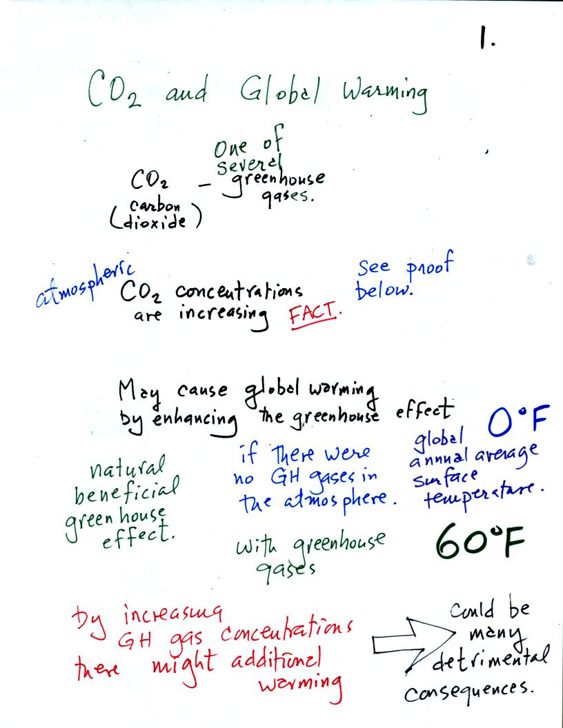
The natural greenhouse effect (i.e. the greenhouse effect
that would be present on earth without the influence of humans) is
beneficial . The
average global annual surface temperature on earth without
greenhouse
gases
would be about 0o F. The presence of greenhouse gases
raises this average to about 60o F.
An increase in concentrations of greenhouse gases in the
atmosphere, due to human activities, could enhance the greenhouse
effect
and cause additional warming. This then could have many
detrimental effects such as
melting
polar ice and causing a rise in sea level and
flooding of coastal areas, changes in weather patterns and changes in
the frequency and severity of storms.
Some of the evidence for increasing CO2 concentration is
shown in
the two
graphs below.
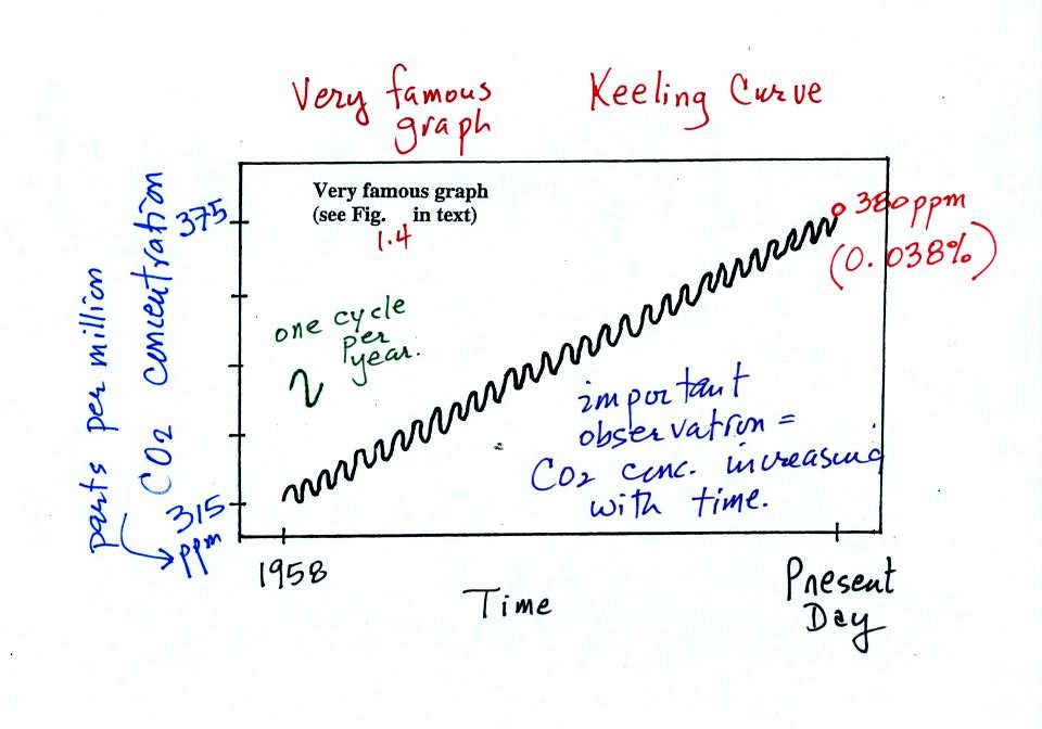
The "Keeling" curve shows measurements of CO2
that
were begun
in 1958 on top of the Mauna Loa volcano in Hawaii. Carbon dioxide
concentrations have increased from 315 ppm to about 380 ppm between
1958 and the present day. The small wiggles (one wiggle per year)
show that CO2
concentration
changes slightly during the year.
Once scientists saw this data they began to wonder about how
CO2
concentration might have been changing prior to 1958. But how
could you now, in 2007, go back and measure the amount of CO2
in the
atmosphere in the past? Scientists have found a very clever way
of
doing just that. It involves coring down into ice sheets that
have
been building up in Antarctica and Greenland for hundreds of thousands
of years.
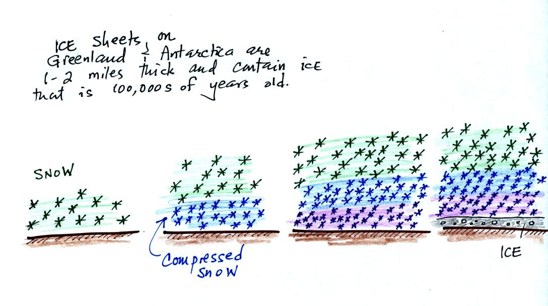
As layers of snow are piled on top of each other year
after
year, the
snow at the bottom is compressed and eventually turns into a thin layer
of
solid
ice. The ice contains small bubbles of air trapped in the snow,
samples of the atmosphere at
the time the snow originally fell. Scientists are able to date
the ice layers and then
take the air out of these bubbles and measure the carbon dioxide
concentration. This isn't easy, the layers are very thin and the
bubbles are small. It is hard to avoid contamination.
A
book, The Two-Mile Time Machine, by Richard B.
Alley discusses ice cores and climate change. This is one of the
books available for checkout should you decide to write a book report
instead of an experiment report.
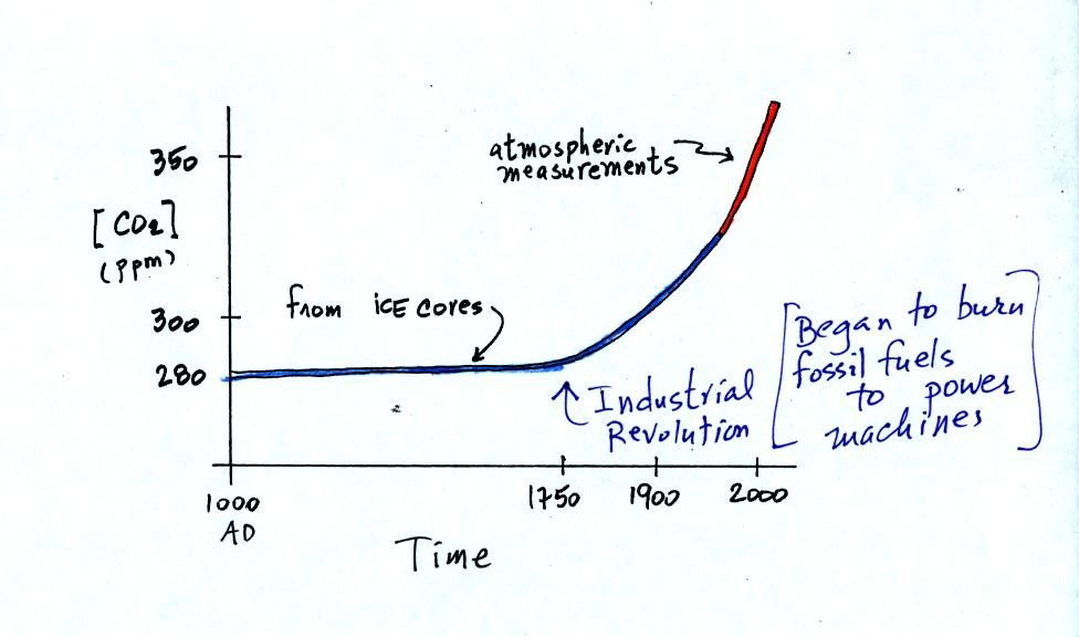
Using the ice core measurements scientists have determined
that
atmospheric CO2 concentration was fairly constant at about
280 ppm
between
1000 AD and the mid-1700s when it started to increase. The start
of rising CO2 coincides with the beginning of the
"Industrial
Revolution."
Combustion of fossil fuels needed to power factories began to add
significant amounts of CO2
to the
atmosphere.
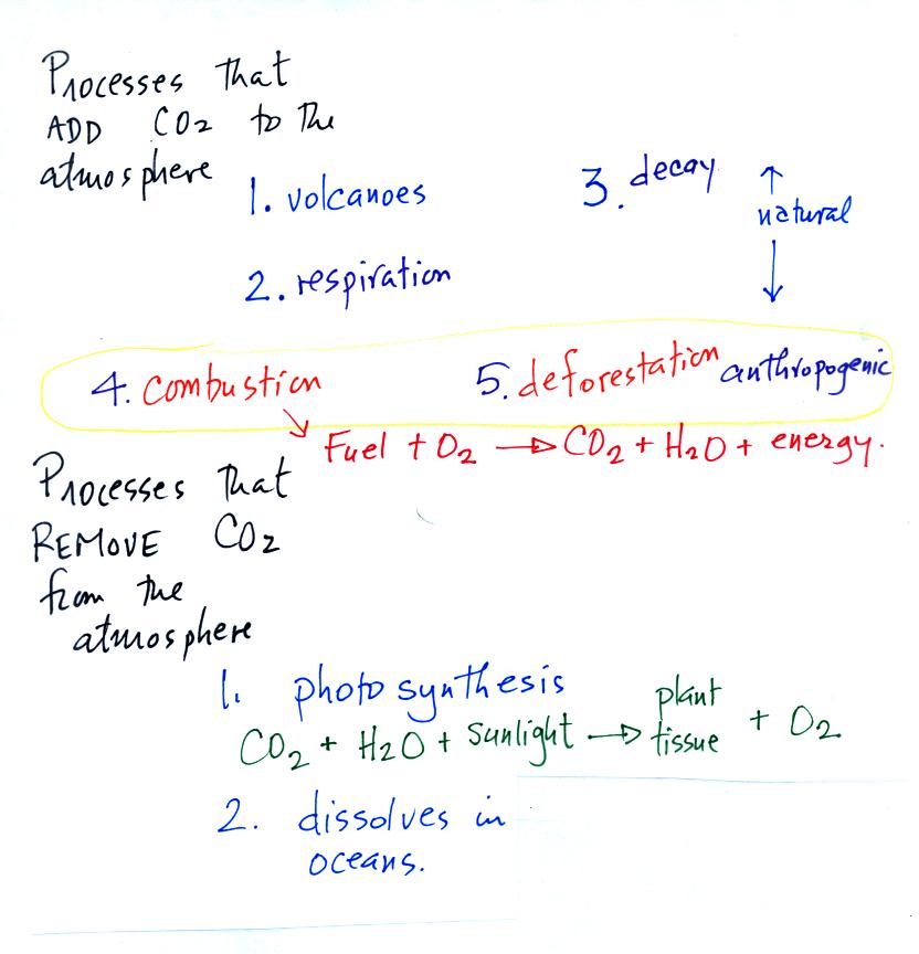
Carbon dioxide is added
to the
atmosphere naturally by respiration (people breathe in oxygen and
exhale carbon dioxide), decay, and volcanoes. Combustion of
fossil fuels, a human activity also addes CO2 to the
atmosphere. Deforestation,
cutting down and killing a tree (or burning the tree) will keep
it from removing CO2 from the air by photosynthesis.
The dead
tree will also decay and release CO2 to the air.
The chemical equation illustrates the combustion of a fossil
fuel. The by products are carbon dioxide and water vapor.
The steam cloud that
you sometimes see come from a rooftop vent or the tailpipe of an
automobile (especially during cold weather) is evidence of the
production of water vapor during the
combustion.
Photosynthesis removes CO2 from the air (photosynthesis adds
oxygen to the air). CO2
also dissolves in
ocean water.
We can use this information to better understand the
yearly
variation in atmospheric CO2
concentration (the "wiggles" on the Keeling Curve).
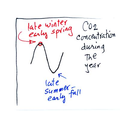
Atmospheric CO2 peaks in the late winter to early
spring. Many
plants die or become dormant in the winter. With less
photosynthesis, more CO2 is added to the atmosphere than can
be
removed. The concentration builds throughout the winter
and reaches a peak value in late winter - early spring. Plants
come back to life at that time and begin to remove carbon dioxide.
In the summer the removal of CO2 by photosynthesis
exceeds
release. CO2 concentration decreases throughout the
summer and
reaches a minimum in late summer to early fall.
To
really understand
why human activities are causing atmospheric CO2
concentration to
increase we need to look at the relative amounts of CO2
being added to
and being removed from the atmosphere (like amounts of money moving
into and out of a bank account and their effect on the account
balance). A simplified version of the carbon cycle is shown below.
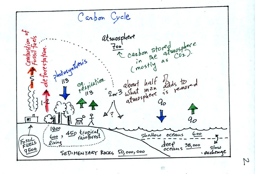
This somewhat confusing figure also requires some
careful examination.
1. Underlined numbers show
the amount of carbon stored in "reservoirs." For example 700
units* of carbon
are stored in the atmosphere (predominantly in the form of CO2,
but
also in small amounts of CH4 (methane),
CFCs
and other gases; carbon is found in each of those
molecules). The other numbers show
"fluxes," the amount of carbon moving into or out of the atmosphere
every
year. Over land, respiration and decay add 113 units* of carbon
to the
atmosphere every year. Photosynthesis (primarily) removes 113
units every year.
2. Note the natural processes
are in balance (over land: 113 units added and 113 units removed, over
the oceans: 90 units added balanced by 90 units of carbon removed from
the atmosphere every year). If these were the only processes present,
the atmospheric concentration (700 units)
wouldn't change.
3. Anthropogenic (man caused) emissions
of
carbon into the air are small compared to natural processes. About
5 units are added during combustion of fossil fuels and 1-2
units are added every year because of deforestation (when trees are cut
down they decay and add CO2 to the air, also because they
are dead they
aren't able to remove CO2 from the air by photosynthesis)
The rate at which carbon is added to the atmosphere by man is not
balanced by an equal rate of removal (2 or 3 units are removed every
year, highlighted in yellow in the figure. The ? refers to the
fact that scientists still don't know precisely how or where this
removal occurs). This small imbalance explains why
atmospheric carbon dioxide concentrations are increasing with time.
4. In the next 100 years or so,
the 7500 units of carbon stored in the fossil fuels reservoir (lower
left
hand corner of the figure) will be added to the air. The big
question is how will the atmospheric
concentration change and what effects will that have?
*units: Gtons (reservoirs) or Gtons/year (fluxes)
Gtons = 1012 metric tons. (1 metric ton is 1000 kilograms or
about 2200
pounds)
So here's
what we know so far:
Atmospheric CO2 concentration was fairly constant between
1000 AD and
the mid
1700s. CO2 concentration has been increasing since the
mid
1700s (other greenhouse gas concentrations have also been
increasing). The concern is that this might enhance or strengthen
the
greenhouse effect and cause global warming.
What has
the temperature of the earth been doing during this period? There
is a two part answer to that question.
First part:
Accurate direct measurements of temperature are available only from the
past
150 years or so. The figure below, redrawn after class for clarity
(top of p. 3 in the photocopied
Class Notes and also Fig. 14.7 in the text) shows how global
average
surface temperature has changed during that time period.
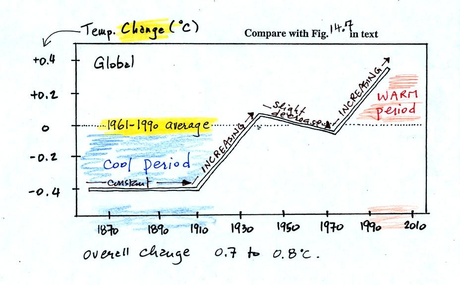
This is
based on actual measurements of temperature made (using thermometers)
at many locations on
land and sea around the globe.
The graph doesn't actually show temperature. It shows how much
different temperatures at various times beween 1860 and 2000 were
compared to the 1961-1990 average. Temperature appears to have
increased 0.7o to 0.8o
C during this
period. The increase hasn't been steady as you might have
expected given
the steady rise in CO2 concentration; temperature even
decreased slightly between 1940 and 1975.
It is very difficult to detect a temperature change this small over
this period of time. The instruments used to measure temperature
have changed. The locations at which temperature measurements
have been made have also changed (imagine what Tucson was like 130
years ago). Average surface temperatures naturally change a lot
from year to year. The year to year variation has been left out
of the figure above so that the overall trend could be seen more
clearly (click here
to see a
different
version of this figure that does show the year to year variation and
the uncertainties in the yearly measurements).
2nd part
Now it would be interesting to know how temperature was changing prior
to the mid-1800s. This is similar to what happened when the
scientists wanted to know what carbon dioxide concentrations looked
like prior to 1958. In that case they were able to go back and
analyze air samples from the past (trapped in bubbles in ice
sheets).
That doesn't work with temperature.
Imagine putting some air in a
bottle, sealing the bottle, putting the
bottle on a shelf, and letting it sit for 100 years. In 2107 you
could take the bottle down from the shelf, carefully remove the air,
and measure
what the CO2 concentration in the air had been in 2007 when the air was
sealed in the bottle. You couldn't, in 2107, use the air in the
bottle to determine what the temperature of the air was when it was
originally put into the bottle in 2007.
You need to use proxy data.
You need to look for something else whose presence, concentration, or
composition depended on
the temperature at some time in the past.
Here's an example.
Let's say you want
to determine how many students are living in
a house near the university.
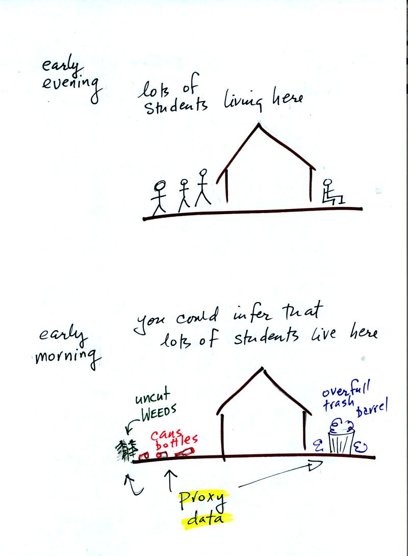
You
could walk by the house late in
the afternoon when the students might be outside and count them.
That
would be a direct measurement (this would be like measuring temperature
with a thermometer). There could still be some errors in your
measurement (some students might be hidden inside the house, some of
the people outside might not live at the house).
If you were to walk by early in the morning it is likely that the
students would be inside sleeping (or in one of the 8 am NATS 101
classes). In that case you might
look for other clues (such as the number of empty bottles in the yard)
that might give you an idea of how many students
lived in that house. You would use these proxy data to come up
with an estimate of the number of students inside the house.
In the case of temperature scientists look at a variety of
things. They could look at tree rings. The width of each
yearly ring depends on the depends on the temperature and
precipitation at the time the ring formed. They analyze
coral. Coral is made up of calcium carbonate, a molecule that
contains oxygen. The relative amounts of the different oxygen
isotopes (atoms of oxygen with different numbers of neutrons in the
nucleus) depends
on the temperature that existed at the time the coral grew.
Scientists can analyze lake bed and ocean sediments. The types
of plant and animal fossils that they find depends on
the water temperature at the time. They can even use the ice
cores. The ice, H2O, contains oxygen and the relative
amounts of
various oxygen isotopes depends on the temperature at the time the ice
fell from the sky as snow.
Using these proxy data scientists have been able to estimate average
surface temperatures for 100,000s of years into the past. The
next figure shows what temperature has been doing since 1000 AD.
This is for the northern hemisphere only, not the globe.
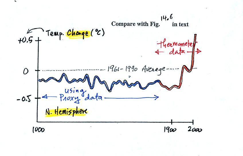
The
blue
portion of the figure shows the estimates of temperature
derived from proxy data. The red portion are the instrumental
measurements made between about 1860 and the present day. There
is also a lot of year
to year variation and uncertainty that is not shown on the figure above
(click here
or see Figure 14.6 in the
text for a more accurate representation of this curve).
It appears that there has been a significant amount of warming that has
occurred in just the last 150 years or so. Many scientists
believe that this warming is a result of the increase in atmospheric
greenhouse gas concentrations. Others suggest that this change in
temperature might be just a natural change in climate (Mother
Nature has
produced much larger changes than we see here though usually on a much
longer time scale), or might be do to other human activities that
affect climate (changing land use).
We've only
considered a small part of a large debate that involves science,
economics, and politics.
Summary (not included in class)
There is general agreement that
Atmospheric CO2 and other greenhouse gas
concentrations are
increasing and that
The earth is warming
Not everyone agrees
on the Causes (natural or manmade) of the warming or
on the Effects that warming will have on weather and
climate in the years to come
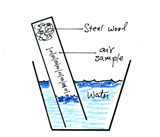
The object
of this experiment is to measure the percentage concentration of the
oxygen in air. Basically a wet piece of steel wool is stuck into
a 100 mL graduated cylinder. The cylinder is turned upside down
and the open end is immersed in a cup of water. The air in the
graduated cylinder is sealed off from the rest of the atmosphere.
The oxygen reacts with the steel wool to form rust and is removed from
the air sample (it turns from a gas and becomes part of the rust, a
solid).
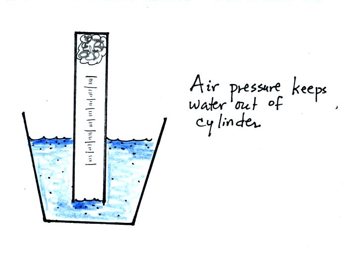
If you simply try to immerse the open end of the cylinder in a cup
of water you would find that the water doesn't enter the
cylinder. Air pressure keeps the water out. You want the
water to enter partway into the cylinder so that the water level can be
read on the cylinder scale.

Note that it isn't that the cylinder is full of air that keeps the
water out (as shown above at left), there's actually a lot of empty
space in the cylinder. Rather it is the fact that the air
molecules are moving around inside the cylinder at 100s of miles per
hour and they strike the water molecules with enough force that the
water can't move into the cylinder.

The solution to this problem is to insert a small piece of
flexible tubing into the cylinder as shown above. If you lower
the cylinder into the water while keeping the two ends of the tubing
out of the water, water will enter the cylinder. When the water
level can be read on the scale (ideally between the 90 and 100 ml
marks), the tubing is removed. This seals off the air sample and
the experiment is underway.
You can carefully rest the cylinder against bottom and side of the
cup. Be sure to tell any friends or roommates to leave your
experiment materials alone.
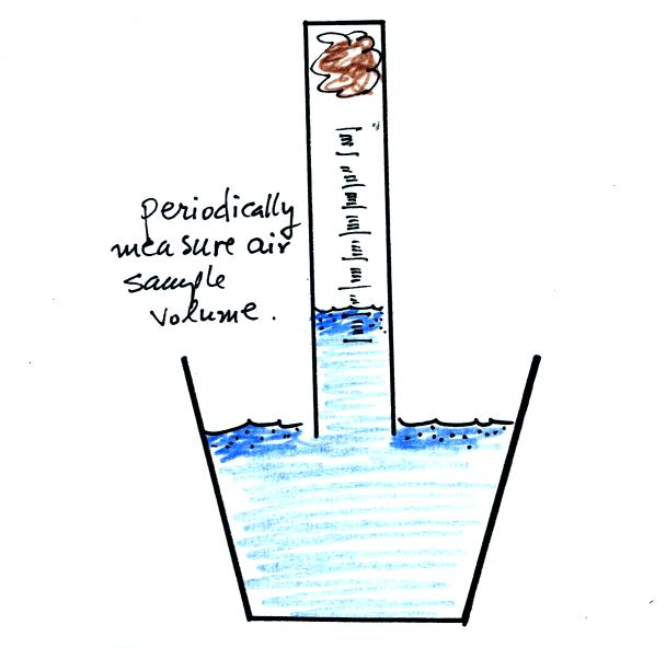
Periodically lift the cylinder just enough to be able to read the
water level. Don't lift the open end of the cylinder out of the
water as this would break the seal and you would need to restart the
experiment (extra pieces of steel wool will be available in class
should this happen). Also make a note of the time.
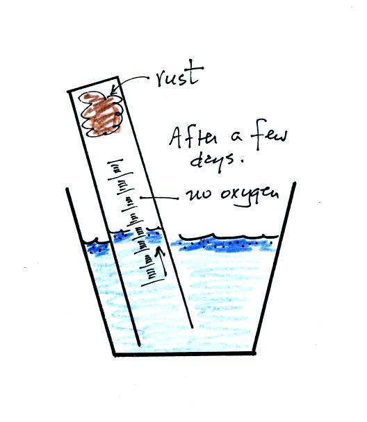
After some time you will notice that the water level doesn't
change between readings. All of the oxygen in the sample has been
removed and the experiment is over. The figure below shows you
one way of removing the steel wool (which should then be
discarded). Return the materials to class and pick up the
supplementary information handout.
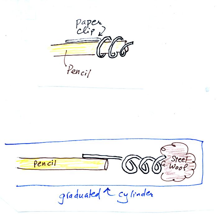
Straighten the paper clip supplied with the experiment and then bend
about 2/3 rds of it around the end of a pencil to form a
corkscrew. Attach the corkscrew to the end of the pencil and then
insert it into the cylinder. With a list twisting the corkscrew will
snag the steel wool and you will be able to pull it out of the cylinder
and dispose of it.